XOR

[Simon Tatham, 2025-02-14]

• Introduction
• XOR in boolean logic
  • What is it?
    • “Exclusive OR”
    • The ‘not equals’ operator
    • Conditional inversion
    • Parity, or sum mod 2
    • Difference mod 2
  • What properties does it have?
• Bitwise XOR on integers
  • Still has all the same properties
  • Bitwise difference
  • Bitwise conditional inverter
  • Addition or subtraction without carrying
• Some applications of XOR
  • Cryptography: combine a plaintext with a keystream
  • Pixel graphics: draw things so it’s easy to undraw them again
  • The “half-adder identity”
    • Averaging two integers
    • Implementing XOR itself
  • Swapping bits in a word
    • Using XOR and shifts
    • Using XOR and just a two-bit word
  • Three XORs make a swap
  • Winning at the game of Nim
• Mathematical concepts that look like XOR
  • Symmetric difference of sets
  • Groups of exponent 2
  • Nim-sum
  • GF(2), the finite field of order 2
    • Linear algebra over GF(2)
      • Error-correcting codes
    • Polynomials over GF(2)
      • CRCs
      • Making larger finite fields
• Footnotes

Introduction

Recently I was called on to explain the ‘XOR’ operator to somebody who vaguely knew of its existence, but didn’t have a good intuition for what it was useful for and how it behaved.

For me, this was one of those ‘future shock’ moments when you realise the world has moved on. When I got started in computers, you had to do low-level bit twiddling to get anything very interesting done, so you pretty much couldn’t avoid learning about XOR. But these days, to a high-level programmer, it’s much more of an optional thing, and you can perfectly well not know much about it.

So I collected some thoughts together and gave a lecture on XOR. Slightly to my own surprise, I was able to spend a full hour talking about it – and then over the course of the next couple of weeks I remembered several other things I could usefully have mentioned.

And once I’d gone to the effort of collecting all those thoughts into one place, it seemed a waste not to write it all down somewhere more permanent. (The collecting is the hardest part!)

So here’s a text version of my XOR talk – or rather, the talk that it would have been if I’d remembered to include everything the first time round.

XOR in boolean logic

We’ll start by looking at XOR as a boolean logic operator, or equivalently a logic gate: a function that takes two individual bits, and outputs a single bit.

What is it?

If I’m going right back to first principles, then I should start by actually defining XOR.

Any boolean function of two inputs can be defined by showing its truth table: for each of the four combinations of inputs, say what the output is. So I’ll start by showing the truth table for XOR.

But just saying what it is doesn’t give a good intuition for what things it’s useful for, or when to use it. So in the next few sections I’ll present a few different ways of thinking about what XOR does.

For such a simple operation, it’s possible to describe what it does in a lot of quite different-looking ways. But all of them are true at once! So you don’t need to keep thinking about XOR as being just one of the following concepts. You can suddenly switch from thinking of it one way to another, any time that’s convenient. Nothing stops being true if you do.

“Exclusive OR”

The X in ‘XOR’ stands for the word “exclusive”. (Some assembly language syntaxes abbreviate it as ‘EOR’ instead, on the grounds that “exclusive” doesn’t actually begin with an X. But most people prefer the X spelling, in my experience.)

In the normal English language, the conjunction ‘or’ has an ambiguity: if I say ‘you can do this or that’, and in fact someone tries to do both this and that, does that count? It depends on the context. A parent telling a child “You can have this dessert or that one” certainly means ‘but not both’ – that’s the whole point. But on the other hand, if the same parent wants the child to do something useful, and says “Do your homework, or tidy your room!”, they’d probably be extra pleased if the child did both.

So, when you want to be clear about which version of ‘or’ you mean, you might say that you’re including the ‘both’ case, or excluding it.

In computing, ‘OR’ as a boolean operator is always taken to mean the inclusive version: A or B or both. And when you want A or B but not both, you talk about exclusive OR.

Looking at the truth tables above, you can see that that’s exactly what the XOR operation is doing:

• If a = 1, or if b = 1, then a XOR b = 1.
• But not both: if a and b are both 1, then a XOR b = 0.

The ‘not equals’ operator

Another way to look at the same truth table is: a XOR b = 1 whenever the inputs a and b are different from each other. If they’re the same (either both 0 or both 1), then a XOR b = 0.

So you could look at a XOR b as meaning the same thing as a ≠ b: it’s a way to compare two boolean values with each other.

Conditional inversion

A third way to look at the same truth table is to consider each value of one of the inputs a, and look at what XOR does to the other variable b in each case:

• If a = 0, then a XOR b is the same thing as just b.
• If a = 1, then a XOR b is the opposite of b: 0 becomes 1 and 1 becomes 0.

So another way to look at the XOR operation is that you’re either going to leave b alone, or invert it (swapping 0 and 1), and a tells you which one to do. If you imagine XOR as a tiny computing device, you could think of the input b as ‘data’ that the device is operating on, and a as a ‘control’ input that tells the device what to do with the data, with the possible choices being ‘flip’ or ‘don’t flip’.

a XOR b means: invert b, but only if a is true.

But the same is also true the other way round, because a XOR b is the same thing as b XOR a. You can swap your point of view to thinking of a as the ‘data’ input and b as ‘control’, and nothing changes – the operation is the same either way round.

That is, a XOR b also means: invert a, but only if b is true!

Parity, or sum mod 2

Here’s yet another way to look at the XOR operation. a XOR b tells you whether an odd number of the inputs are true:

• If a = b = 0, then zero of the inputs are true. 0 is even, and a XOR b = 0.
• If a = 1 and b = 0, or the other way round, then one of the inputs is true. 1 is odd, and a XOR b = 1.
• If a = b = 1, then two of the inputs are true. 2 is even, and a XOR b = 0 again.

Put another way: if you add together the two inputs, and then reduce the result modulo 2 (that is, divide by 2 and take the remainder), you get the same answer as a XOR b.

In particular, if you XOR together more than two values, the overall result will tell you whether an odd or even number of the inputs were 1 – no matter how many inputs you combine.

Difference mod 2

So XOR corresponds to addition mod 2. But it also corresponds to subtraction mod 2, at the same time: if you take the difference a − b and reduce that mod 2, you still get the same answer a XOR b!

• If a = b, then the difference a − b is 0, and so is a XOR b.
• If a ≠ b, then the difference a − b is either +1 or −1. Mod 2, those are the same as each other – they’re both just 1.

What properties does it have?

If you have a complicated boolean expression involving lots of XORs, it’s useful to know how you can manipulate the expression to simplify it.

To begin with, XOR is both commutative and associative, which mean (respectively) that

a XOR b = b XOR a

(a XOR b) XOR c = a XOR (b XOR c)

In practice, what this means is that if you see a long list of values or variables XORed together, you don’t need to worry about what order they’re combined in, because it doesn’t make any difference. You can rearrange the list of inputs into any order you like, and choose any subset of them to combine first, and the answer will be the same regardless.

(This is perhaps most easily seen by thinking of XOR as ‘addition mod 2’, because addition is also both commutative and associative – whether or not it’s mod anything – so XOR inherits both properties.)

Secondly, 0 acts as an identity, which means that XORing anything with zero just gives you the same thing you started with:

a XOR 0 = 0 XOR a = a

So if you have a long list of things XORed together, and you can see that one of them is 0, you can just delete it from the list.

Thirdly, everything is self-inverse¹I apologise for using ‘invert’ and ‘inverse’ in two senses in this article. In boolean logic, ‘inverting’ a signal generally means the NOT operator, interchanging 1 with 0 (or true with false, if you prefer). But in mathematics, an ‘inverse’ is a value that cancels out another value to get you back to the identity, in a way which varies depending on the operation you use to combine them (if you’re talking about addition it’s −x, and for multiplication it’s 1/x). I hope that everywhere I’ve used the word at all it’s clear from context which sense I mean it in.1: if you XOR any value with itself, you always get zero.

a XOR a = 0

One consequence of this is that if you have a long list of variables being XORed together, and the same variable occurs twice in the list, you can just remove both copies. Anything appearing twice cancels out. For example, the two copies of b can be removed in this expression:

a XOR b XOR c XOR b = a XOR c

Another consequence is that if you have a value a XOR b, and you want to recover just a, you can do it by XORing in another copy of b (if you know it), to cancel the one that’s already in the expression. Putting something in a second time is the same as removing it:

(a XOR b) XOR b = a XOR (b XOR b) = a XOR 0 = a

Bitwise XOR on integers

Now we’ve seen what XOR does on individual bits, it’s time to apply it to something larger.

To a computer it’s most natural to represent an integer in binary, so that it looks like a string of 0s and 1s. So if you have two integers, you can combine them bitwise (that is, ‘treating each bit independently’) using a logical operation like XOR: you write the numbers in binary one above the other²What if the integers are negative? Normally, in the finite integer sizes that computers handle in hardware, negative integers are represented in two’s complement, i.e. mod 2ⁿ. So −1 is the integer with all bits 1, for example. There’s a reasonably natural way to extend this to arbitrarily large integers, by pretending the string of 1 bits on the left goes all the way to infinity (and it can even be made mathematically rigorous!). In this view, the XOR of two positive numbers, or two negative numbers, is positive, because at a high enough bit position each bit is XORing two 0s or two 1s; but the XOR of a positive and negative number is negative, because sooner or later you’re always XORing a 0 with a 1 bit. Some languages, such as Python, actually implement this – you can try it out at the interactive prompt!2, and set each output bit to the result of combining the corresponding bits of both input numbers via XOR.

Here are a couple of examples, one small and carefully chosen, and the other large and random-looking:

The small example contains one bit for each element of the XOR truth table. If you look at vertically aligned bits in the binary column of the table, you’ll see that in the rightmost place both a and b have a 0 bit; in the leftmost place they both have a 1 bit; in between, there’s a position where only a has a 1, and one where only b has a 1. And in each position, the output bit is the boolean XOR of the two input bits.

Of course, this idea of ‘bitwise’ logical operations – taking an operation that accepts a small number of input bits, and applying it one bit at a time to a whole binary integer – is not limited to XOR. Bitwise AND and bitwise OR are also well defined operations, and both useful. But this particular article is about XOR, so I’ll stick to that one.

Still has all the same properties

Earlier I discussed a number of mathematical laws obeyed by the one-bit version of XOR: it’s commutative, associative, has 0 as an identity, and every possible input is self-inverse in the sense that XORing it with itself gives 0.

In the bitwise version applied to integers, all of these things are still true:

• a XOR b = b XOR a for any integers a and b
• (a XOR b) XOR c = a XOR (b XOR c) similarly
• a XOR 0 = 0 XOR a = a, where 0 means the integer zero, i.e. with all its binary bits 0
• a XOR a = 0

So if you have a complicated expression containing bitwise XORs, you can simplify it in all the same ways you could do it with single-bit XORs.

Bitwise difference

With individual bits, I said earlier that a XOR b means the same thing as a ≠ b: given two input bits, it returns 1 if the bits are different from each other, and 0 if they’re the same.

Of course, applied bitwise to whole integers, this is true separately in every bit position: each bit of the output integer tells you whether the two corresponding input bits were unequal.

So if a = b, then a XOR b = 0. And if a ≠ b, then a XOR b ≠ 0, because two unequal integers must have disagreed in at least one bit position, so that bit will be set in their XOR.

So in some sense you can still use bitwise XOR to tell you whether two entire integers are equal: it’s 0 if they are, and nonzero if they’re not. But bitwise XOR gives you more detail than that: it also gives you a specific list of which bit positions they differ in.

Bitwise conditional inverter

I also said earlier that you could see XOR as a ‘conditional inversion’ operator: imagine one input b to be ‘data’, and the other input a to be a ‘control’ input that says whether you want to flip the data bit.

Applied bitwise to whole integers, this is still true, but more usefully so: the control input a says which data bits you want to flip.

For example, in the Unicode character encoding (and also in its ancestor ASCII), every character you might need to store in a string is represented by an integer. The choice of integer encodings has some logic to it (at least in places). In particular, the upper-case Latin letters A, B, C, …, Z and their lower-case equivalents a, b, c, …, z have encodings that differ in just one bit: A is 65, or binary 01000001, and a is 97, or binary 01100001. So if you know that a character value represents a Latin letter³Of course, this doesn’t apply to all Unicode characters! Most don’t have a concept of upper or lower case at all. And unfortunately, this rule isn’t even obeyed by all of the characters that do. It was consistently true in ASCII, and in some of the descendants of ASCII, but Unicode as a whole wasn’t able to stick 100% to the principle. If you take this too far, you might get strange ideas, like the lower-case version of the car emoji being a ‘no pedestrians’ sign: >>> chr(ord('🚗') ^ 32)
'🚷'3, you can swap it from upper case to lower case or vice versa by flipping just that one bit between 0 and 1.

And you can do that most easily, in machine code or any other programming language, by XORing it with a number that has just that one bit set, namely binary 00100000, or decimal 32. For example, in Python (where the ^ operator means bitwise XOR):

>>> chr(ord('A') ^ 32)
'a'
>>> chr(ord('x') ^ 32)
'X'

Of course, the other thing I said earlier also applies: it doesn’t matter which of the inputs to XOR you regard as the data, and which as the control. The operation is the same both ways round.

In particular, suppose you’ve already XORed two values a and b to obtain a number d that tells you which bits they differ in. Then you can turn either of a or b into the other one, by XORing with the difference d, because that flips exactly the set of bits where a has the opposite value to b.

In other words, these three statements are all equivalent – if any one of them is true, then so are the other two:

a XOR b = d
a XOR d = b
b XOR d = a

Addition or subtraction without carrying

Another thing I mentioned about XOR on single bits is that it corresponds to addition mod 2, or equivalently, subtraction mod 2.

That isn’t quite how it works once you do it bitwise on whole words⁴I suppose, technically, you could argue that it is still literally true that a XOR b, a + b, and a − b are all congruent to each other mod 2, because all that means is that they all have the same low-order bit, which they do. But that isn’t a particularly useful thing to say, because it ignores the way all the higher-order bits do something completely different!4. Each individual pair of bits is added mod 2, but each of those additions is independent.

One way to look at this is: suppose you were a schoolchild just learning addition, and you’d simply forgotten that it was necessary to carry an overflowed sum between digit positions at all. So for every column of the sum, you’d add up the input digits in that column, write down the low-order digit of whatever you got, and ignore the carry completely.

If this imaginary schoolchild were to do this procedure in binary rather than decimal, the operation they’d be performing is exactly bitwise XOR! Bitwise XOR is like binary addition, without any carrying.

Later on I’ll show an interesting consequence of this, by considering what does happen to the carry bits, and how you can put them back in again afterwards. There’s also a mathematically meaningful and useful interpretation of the corresponding ‘carryless’ version of multiplication, in which you make a shifted version of one of the inputs for each 1 bit in the other, and then add them together in this carryless XOR style instead of via normal addition.

Some applications of XOR

Now we’ve seen what XOR is, and a few different things it’s like, let’s look at some things it’s used for.

Cryptography: combine a plaintext with a keystream

XOR is used all over cryptography, in many different ways. I won’t go into the details of all of those ways – I’m sure I don’t even know all of them myself! – but I’ll show a simple and commonly used one.

Suppose you have a message to encrypt. One really simple thing you could do would be to take an equally long stream of random-looking data – usually known as a ‘keystream’ – and combine the two streams, a byte or a word at a time, in some way that the receiver can undo. So if your message was “hello”, for example, you might simply transmit a byte made by combining “h” with keystream byte #1, then one that’s “e” combined with keystream byte #2, and so on.

This seems absurdly simple – surely real cryptography is terrifyingly complicated compared to this? But it really is a thing that happens. As long as each byte is combined with the keystream byte in a way that makes it possible to recover the original byte at the other end, this is a completely sensible way to encrypt a message⁵However, encrypting the message is only half the story. Given a good-quality keystream, this technique is good enough to assure confidentiality, meaning that an eavesdropper can’t find out what you’re saying. But it doesn’t do one single thing to ensure integrity, meaning that if your message is modified by an attacker, the receiver can detect the tampering and know not to trust the modified message. Integrity protection is a completely separate problem. A common mistake in novice cryptosystem design is to leave it out, assuming that if nobody can figure out what the message says, then “surely” nobody can work out how to tamper with it in a useful way either. Even with more complicated encryption methods than what I’m describing here, this never goes well!5!

That’s not to say that there isn’t terrifyingly complicated stuff somewhere in the setup. But in this particular context, the complicated part is in how you generate your stream of random-looking bytes; the final step where you combine it with the message is the easy part. One option is for your keystream to be a huge amount of genuinely random data, as big as the total size of all messages you’ll ever need to send; this is known as a ‘one-time pad’, and is famously actually unbreakable – but also amazingly impractical for almost all purposes. More usually you use a stream cipher, or a block cipher run in a counter mode, to expand a manageably small actual key into a keystream as long as you need.

Anyway. I’ve so far left out the detail of exactly how you “combine” the keystream with the message. But given the subject of this article, you can probably guess that it’s going to be XOR.

XOR isn’t the only thing that would work. If your message and your keystream are each made of bytes, then there are plenty of other ways to combine two bytes that let you recover one of them later. For example, addition mod 2⁸ would be fine: you could make each encrypted byte by adding the message byte and keystream byte, and then the receiver (who has access to exactly the same keystream) would subtract the keystream byte from the sum to recover the message byte.

But in practice, XOR is generally what’s used, because it’s simpler. Not so much for software – CPUs generally have an ‘ADD’ instruction and an ‘XOR’ instruction which are just as fast and easy to use as each other – but encryption is also often done in hardware, by specially made circuitry. And if you’re building hardware, addition is more complicated than XOR, because you have to worry about carrying between bit positions, which costs more space on the chip (extra logic gates) and also extra time (propagating signals from one end to the other of the addition). XOR avoids both problems: in custom hardware, it’s far cheaper.

(It’s also very slightly more convenient that the sender and receiver don’t have to do different operations. With XOR, the sender who applies the keystream and the receiver who takes it off again are both doing exactly the same thing, instead of one adding and the other subtracting.)

Pixel graphics: draw things so it’s easy to undraw them again

Let’s set the wayback machine to the mid-1980s, and go back in time to when computers were smaller and simpler (at least, the kind you could afford to have in your home). Home computer graphics systems stored a very small number of bits for each pixel on the screen, meaning that you could only display a limited number of different colours at a time; and even with that limitation on framebuffer size, home computers had so little RAM in total that it was a struggle to store two entire copies of what was displayed on the screen and still have enough memory for anything else (like whatever program was generating that screenful of graphics).

In an environment limited like that, what do you do if you want to draw an object that appears and disappears, or that moves around gradually?

If your moving object is opaque, then every time you ‘undraw’ it, you have to restore whatever was supposed to be on the screen behind it. That means you have to remember what was behind it – either by storing the actual pixels, or by storing some recipe that knows how to recreate the missing patch of graphics from scratch. Either one costs memory, and the second option probably costs time as well, and you don’t have a lot of either to spare.

Nevertheless, you do that when you really have to. But when you don’t have to, it’s always helpful to take shortcuts.

So one common graphical dodge was: don’t make graphical objects opaque if you don’t have to. Any time you can get away with it, prefer to draw a thing on the screen in a way that is reversible: combine each pixel M of the moving object with the existing screen pixel S, in such a way that you can undo the operation later, recovering the original screen pixel S from the combined value C by remembering what M was.

As in the previous section, there are plenty of ways to do this in principle. You could imagine treating the bits of each pixel as an n-bit integer for some small n, and doing addition and subtraction on them (again, mod 2ⁿ). For example, you could draw by addition, setting C = S + M, and undraw by subtraction to recover S = C − M.

But these systems typically had far fewer than 8 bits per pixel, so each byte of the screen would have more than one pixel packed into it. Or, worse, the screen might be laid out in ‘bit planes’, with several widely separated blocks of memory each containing one bit of every pixel. Doing ordinary addition on the pixel values is very awkward in both cases.

In particular, consider the first of those possibilities, where you have several pixels packed into a byte. Suppose the 8 bits of the byte are treated as two 4-bit integers, or four 2-bit integers. In order to do parallel addition of each of those small chunks, you can’t use the normal CPU’s addition instruction, because a carry off the top of one pixel value propagates into the next, causing unwanted graphical effects. So you’d somehow need to arrange to suppress the carry between pixels, but leave the carry within a pixel alone.

So it’s much easier not to try this in the first place. Combining the pixel values via XOR instead of addition means that you automatically avoid carries between pixels, because there are no carries at all. This is also more convenient in the ‘bit plane’ memory layout, because each bit of a pixel is treated independently; if you tried to do ordinary addition in that situation, you’d have to make extra effort to propagate carries between corresponding bits in each bit plane.

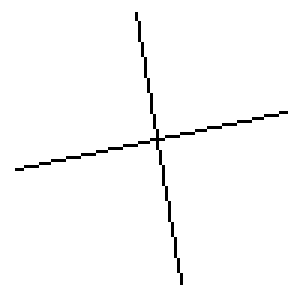
Here’s a simple example, in which two lines have been drawn crossing each other. You can see that in the second diagram, drawn using XOR, there’s a missing pixel at the point where the two lines cross. That pixel is part of both lines, so it’s been drawn twice. Each time it was drawn, the pixel value flipped between black and white, so drawing it twice sets it back to the background colour.

That missing pixel looks like a tiny blemish. The first version of the picture looks nicer. But it makes it harder to undraw one of those lines later. If you just undraw it by setting all the pixels of one line back to white, then you leave a hole in the remaining line. And if you don’t want to leave a hole, then you need some method of remembering which pixel not to reset to white.

In the XOR version of the picture, it’s the easiest thing in the world to undraw one line and leave the other one undamaged. Simply draw the line again that you want to undraw. Putting a second copy of something into an XOR combination is the same as removing it. This kind of graphical ‘blemish’ was considered a reasonable price to pay, in situations where efficient undrawing and redrawing was needed.

Most types of 1980s home computers had an option to draw in XOR mode, for this kind of reason. It was one of the easiest ways for a beginning computer programmer to draw pretty animations. A common type of demo was to simulate two points moving around the screen along a pair of independent paths, and draw a line between the two points at each moment – but to allow the previous few versions of the line to persist as well as the latest one, undrawing each one after it had been on the screen for a few frames.

Here’s an example of the kind of thing. In this example each end of the line is following a path given by a different Lissajous curve:

Because we’re drawing the lines in XOR mode, the procedure for turning each frame of this animation into the next involves drawing only two lines: the new one that we’re adding at the leading edge of the motion, and the one that’s about to vanish from the trailing edge. So the program only has to remember the endpoint coordinates of the 10 (or however many) lines it currently has on screen – or perhaps not even bother with that, and just recalculate the (n − 10)th coordinate in each frame to work out what line to undraw.

So this lets you produce pretty and interesting results, with almost no memory cost (you don’t have to store extra copies of lots of pixels). It uses very little CPU as well (you don’t have to redraw all the lines in every frame, only the ones you’re adding and removing), which makes the animation able to run faster.

This style of animation was a common thing for beginning programmers to play with, but it was also used by professionals. Perhaps most famously, a moving line drawn in this style acted as the main antagonist of the 1981 video game Qix.

Even in the 1990s, with slightly larger computers, XOR-based drawing and undrawing was still a useful thing: in early GUI environments like the Amiga, when you dragged a window around the screen with the mouse, the system didn’t have enough CPU to redraw the entire window as you went. Instead it would draw an outline frame for where the window was going to end up, and once you’d put it in the right place, you’d let go of the mouse button and the window would be properly redrawn in the new location, just once. And again the outline frame would be drawn using XOR, so that it didn’t cost extra memory to remember how to undraw it on each mouse movement.

But going back to the above animation: if you watch it carefully, you might notice that when the moving endpoints change direction and a lot of the lines cross each other, the missing pixels at the crossing points give rise to a sort of interference effect. Those missing pixels started off as a necessity to save memory, but it turns out they’re also quite pretty in their own right.

Another favourite kind of 1980s graphical program for beginners was to explore those interference patterns more fully. Here’s an image created by drawing a sequence of lines, all with one endpoint in the bottom left corner of the frame, and with the other endpoints being every single pixel along the top row. In ordinary drawing mode this would just be a slow way to fill in a big black triangle. But in XOR mode, the lines interfere with each other wherever more than one of them passes through the same pixel:

That’s actually interesting, and it takes some time to work out what’s going on!

The topmost row is all black, because every pixel on that row is drawn just once, by the line whose endpoint is at exactly that position. But half way up, there’s an all-white row, because the n lines in the image have only n / 2 pixels to pass through on their way to the top row. So you get two lines passing through each pixel, so every pixel is drawn exactly twice, and cancels out back to white. Similarly, a third of the way up there’s another black row where every pixel is drawn exactly three times, and so on. And generally, 1 / n of the way from bottom to top, you expect an all-black row if n is odd, or an all-white row if n is even.

But in between those 1 / n rows, something much more interesting happens, when the number of lines going through each pixel isn’t the same everywhere on the row. Those interference patterns are related to the distribution of rounding errors in computing the horizontal position of each pixel of the line.

I’ll end this section with a question that I don’t know the answer to. Suppose you continue this interference-pattern drawing further to the right, past the point where the line slopes at 45°:

At the 45° mark, something changes fundamentally. Those horizontal black and white stripes have changed direction, and now they’re sloping at what looks like a constant angle.

I understand why something has changed. In this style of pixelated line drawing, a line that’s closer to horizontal than vertical can have multiple pixels on each row, and only one in each column, whereas if it’s closer to vertical than horizontal, it’s the other way round. So that’s a good reason why the picture should look fundamentally different in some way on opposite sides of the 45° line.

But why does that give rise to a consistently sloping set of coloured stripes, and not any other kind of weird effect? I’ve never sat down and worked that one out.

The “half-adder identity”

I said in a previous section that one way to look at the expression a XOR b is that it’s the remainder mod 2 of a + b. Another way to say that is that it’s the low-order binary digit of a + b.

What about the high one?

To answer that, let’s start with a truth table:

Here, I’ve shown the actual value of the sum a + b for each possible input. Then I’ve written each of those values in binary, so that 0 and 1 become 00 and 01, and 2 becomes 10. You can see that the high bit of the sum is only 1 if both inputs are set.

In other words: the low bit of a + b is a XOR b, and the high bit is a AND b. In other words, a + b = (a XOR b) + 2 × (a AND b).

That makes sense, if a and b are individual bits. What if we did the same operations bitwise, on whole integers?

If a and b are 32-bit integers (for example), then we’ve already seen above that a XOR b is the integer you get if you add the bits in each position, but not carrying from one bit position to the next. But also, a AND b is an integer consisting of exactly those carry bits: the nth bit of a AND b is 1 precisely when a carry bit should have been generated in that bit position but wasn’t.

If there should have been a carry bit out of the nth place, then it should have been added to the (n + 1)st place. But it’s not too late – we can add it anyway!

In fact, the above equation for single bits a, b is still true⁶If you’re mathematically minded and still don’t find this instantly obvious, you might want to try actually proving it. I leave this mostly as an exercise for the reader, but a hint would be: break down each of the input integers a and b as the sum of terms like 2ⁿa_n (each one being an individual bit of one of the inputs times a power of 2), and collect together the terms on each side that involve the same n.6, even when a, b are whole integers, and the XOR and AND operators are bitwise:

a + b = (a XOR b) + 2 × (a AND b)

Just to show it in action, here’s a demonstration set of values, chosen so that the binary values cover a lot of possible bit combinations, but the decimal values make it immediately clear that the final line is also a + b:

I think of this as the “half-adder identity” (although as far as I know that’s not a standard name). The name comes from the hardware design concept of a “half-adder”, which is a small logic component consisting of just an AND and XOR gate, doing addition of two bits in hardware:

It’s called a half adder because in order to do full binary addition you need two of these per bit, because you have to add three input bits: two from the input integers and one carried from the bit position to the right. So you build a full adder out of two half-adders, one adding a to b and the second adding the sum of those two to c, with one extra gate⁷The extra gate that combines the carry bits can be either an OR gate or an XOR gate, whichever is easier. It doesn’t matter which, because the two types of gate only disagree in the case where both their inputs are 1, and in this circuit, that can’t happen! If the carry from the first half-adder is 1, then its other output must be 0, which means there’s no carry from the second half-adder.7 to combine the two carry bits:

“But hang on,” you might be thinking. “If you need two half-adders per bit to do a full addition, how is that ‘half-adder identity’ of yours getting away with just one pair of AND and XOR operations per bit?” Or you might think: “You’ve generated an output carry from each bit position, but where have you handled the input carry?” Or you might think “Hang on, how do you arrange for a carry in the lowest bit of the addition to potentially propagate all the way up to the top, when the only left shift in this expression moves data by only one bit?”

The answer to all three questions is: because of the + sign on the right-hand side of the identity. After we compute the outputs of one half-adder on each pair of input bits, producing a word full of low bits and a word full of carries … we recombine the two words using an addition. That’s what finishes the job of propagating carries.

In other words, unlike the hardware half-adder, the “half-adder identity” doesn’t build an addition out of only simpler operations. It builds an addition out of two simpler operations and an addition.

“Well, in that case,” you might think, “isn’t it a complete cheat, and not useful for anything?”

Not quite! It’s true that this identity is not often useful. But ‘not often’ isn’t ‘never’, and in unusual circumstances there are uses for it.

Averaging two integers

Here’s one occasional use for the half-adder identity.

Suppose you need to calculate the average of two integers, each the size of your CPU’s registers (let’s say, 32 bits). In other words, you want to add two integers, and then divide by 2 (or, equivalently, shift right by 1 bit).

But adding two 32-bit integers makes a 33-bit sum, which doesn’t fit in your register. If you just do the simple thing – add and then shift – then you potentially get the wrong answer, because the topmost bit has been lost in between the addition and the right shift.

Most CPUs have a good answer to this. The add instruction can (perhaps optionally) set a ‘carry flag’ to indicate whether a 1 bit was carried off the top of an addition; also, there’s usually a special form of right shift by 1 bit that brings the carry bit back in to the top of the word. (On Arm, that instruction is called RRX; on x86, RCR.) So the way to average two numbers without an overflow problem is to do ADD followed by RRX.

But a few CPUs can’t do it that way. Some architectures don’t have a carry flag at all, or indeed any other flags: for example, MIPS, RISC-V, and the historic DEC Alpha. In other situations, there is a carry flag, but no convenient RRX instruction, so that it would take a lot of effort to recover the carry bit and put it at the top of the shifted-right word; for example, the initial versions of Arm’s space-efficient “Thumb” instruction set discarded the RRX instruction, simply because there wasn’t room for everything.

So, if you can’t do ADD and RRX, how do you most efficiently compute your average?

The half-adder identity provides the answer. If the sum of the two inputs is expressed like this (with the << operation meaning ‘shift left’) …

a + b = (a XOR b) + (a AND b) << 1

… but what you want is the same sum shifted right by one bit, then all you have to do is to shift the XOR term right, instead of the AND term left:

(a + b) >> 1 = (a XOR b) >> 1 + (a AND b)

Implementing XOR itself

Also on the theme of ‘compensating for missing features of your CPU’, here’s another thing you can do with the half-adder identity.

In the 1970s, Data General made a CPU with such a small instruction set that it didn’t even implement the bitwise XOR operation – it had AND, but not XOR. On that CPU, what would you have done if you needed XOR?

The answer is to use the half-adder identity in reverse! Instead of starting from a XOR b and making a + b, do it the other way round. Given the equation

a + b = (a XOR b) + 2 × (a AND b)

you can rearrange it to get

a XOR b = (a + b) − 2 × (a AND b)

So if you have addition and bitwise AND, you can build XOR out of them!

(Exercise for the reader: you can also make bitwise OR in the same way, by removing the “2 ×” in the expression – subtract (a AND b) without doubling it first.)

Swapping bits in a word

Suppose you have a collection of bits packed into an integer, and you want to swap the positions of two of them. What’s the best way?

There’s no one answer to that question, because a lot depends on what hardware you’re doing it on (and what useful capabilities it has), and also, on what else you want to do at the same time. For example, swapping a lot of pairs of bits can often be done more efficiently than by swapping one pair at a time. So this is one of these simple-looking questions that becomes surprisingly complicated if you add “… and do it absolutely as fast as possible” to the requirements.

But more than one of the good techniques for solving this problem are based on XOR, because you can divide the problem into two essential cases:

• If the two bits you want to swap are both 0, or both 1, then swapping them makes no difference anyway. So in that situation, you don’t need to do anything at all.
• If one of the bits is 0 and the other is 1, then swapping them is the same as inverting each one.

In other words, a reasonable strategy is: first find out if the bits are different, and then, if so, invert both.

Both of those are applications of XOR. If you XOR the two bits with each other, that will give you 1 if they’re different. And then you can use that value as input to another XOR, using it as a ‘controlled bit flip’ to invert both bits, but only if they were different to start with.

Using XOR and shifts

Here’s a piece of pseudocode that uses that principle to swap two bits. It assumes that pos0 and pos1 are the positions of the two bits to be swapped, with 0 meaning the units bit, 1 the bit to its left, and so on. It also assumes that pos1 > pos0.

# Constants derived from pos0 and pos1
bit0 = (1 << pos0)      # an integer with just the bit at pos0 set
distance = pos1 - pos0  # distance between the two bits

# Computation starting from the input value
diff_all = input XOR (input >> distance)
diff_one = diff_all AND bit0
diff_dup = diff_one XOR (diff_one << distance)
output = input XOR diff_dup

(If you need to swap the same pair of bit positions in a lot of inputs, the first two lines can be precomputed just once and reused.)

The first value we compute, diff_all, is made by shifting the input right by the distance between the two bit positions. So each bit of diff_all tells you the difference between a pair of the input bits separated by that distance.

But we’re only interested in one particular pair of the input bits. So next we compute diff_one, which uses bitwise AND to pick out just a single bit of diff_all. This will be 0 if the two bits we want to swap are the same; if they’re different, it will be equal to bit0 (i.e. it will have a single bit set at position pos0).

If we XORed that value back into input, it would conditionally flip the lower of the two bits we want to swap. But we want to conditionally flip both of them. So now we duplicate the useful bit of diff_one into the other bit position, by shifting it left by the distance between the two bits, and combining that with diff_one itself to get diff_dup. This has a 1 in both of the target bit positions if the two bits need to be flipped, and is still all 0 otherwise.

So now, XORing that into the input will flip both bits if necessary, and leave them alone otherwise.

This looks like a lot of effort to swap two bits. But one nice thing about it is that it’s just as easy to swap lots of pairs of bits, if every pair is the same distance apart. (That is, swapping bit i with bit i + d, for multiple different values of i but the same d every time.) In that situation, the only thing you need to change is the step that makes diff_one from diff_all: instead of ANDing with a one-bit constant, AND with a multiple-bit constant, containing the low bit of every pair you want to swap.

Why might you want to do that in turn? Because there’s a general technique called a Beneš network which lets you encode a completely arbitrary permutation in the form of a series of stages, with each stage swapping a lot of pairs of things separated by the same distance. The distances iterate through powers of 2 and then back again: for example, you might do a set of swaps with distances 16, 8, 4, 2, 1, 2, 4, 8, 16. (Or the other way round if you prefer – it doesn’t really matter what order you go through the distances in.) So if you want to permute the bits of a word in a completely arbitrary way, a computational primitive that swaps a lot of bits at equal separation is just what you want for each stage of a Beneš network.

Using XOR and just a two-bit word

In the simpler case where you’re only swapping a single pair of bits, here are a couple of simpler (therefore faster) techniques.

Suppose that you have an integer called bits, which has exactly two bits set, at the positions you want to swap. What happens if you make the bitwise AND of that value with your input? There are three possibilities:

• (input AND bits) = 0. Both bits are 0, so you don’t need to do anything to swap them.
• (input AND bits) = bits. Both bits are 1, so you still don’t need to do anything.
• Otherwise, the two bits have different values, so you can swap them by XORing the input with bits.

On several CPU architectures this kind of test is easier than doing the full business above with shifts – especially because you don’t need the input bit positions specified in multiple ways. For example, many CPU architectures would let you do something like this (though the syntax of the instructions would vary)

  tmp = input AND bits         # zero if both bits are 0
  if tmp == 0, jump to ‘done’  # in which case we have no work to do
  tmp = tmp XOR bits           # now zero if both bits are 1
  if tmp == 0, jump to ‘done’  # so again we have nothing to do
  input = input XOR bits       # in any other case, flip both bits
done:

You could typically do this with about five instructions, because CPUs will typically set a flag as a side effect of each AND or XOR operation to tell you whether the result was zero. Or, if not that, they might have a single instruction to jump to a different location depending on whether a register is zero.

On the 32-bit Arm architecture you can do this in just three instructions, because you don’t need the jumps: instead, you can make the two XOR operations conditional, because 32-bit Arm generally lets you make an instruction conditional on the current CPU flags without needing a separate branch instruction to skip past it.

And on x86, you can also do it in three instructions for a completely different reason. x86 has an even stranger processor status flag called the ‘parity flag’. This is set whenever the result of an operation has an odd number of 1 bits. And in this situation, that’s exactly the case where you need to flip the bits! So you don’t need to test separately for the ‘both bits 0’ and ‘both bits 1’ cases: they can be tested together, by checking if the parity flag says there were an even number of 1 bits in the result of the AND operation.

  ANDS    tmp, input, bits
  EORSNE  tmp, tmp, bits
  EORNE   input, input, bits

  TST     input, bits
  JPE     done
  XOR     input, bits
done:

Three XORs make a swap

In a computer program, how do you swap two numbers?

It depends on the platform. Some programming languages have a dedicated function for it, like C++’s std::swap. Others have a convenient syntax for assigning multiple variables at once: in Rust you can write (a, b) = (b, a) (assuming the variables are mut), and in Python the same thing works without even needing the brackets. Even some machine languages support swapping two registers: for example, x86 has the XCHG (exchange) instruction.

But suppose you’re in a simpler language without any of those features, like C. Or suppose you’re programming machine code on an architecture without a ‘swap two registers’ instruction⁸There is an Arm instruction called SWP for ‘swap’, but it’s not what you want for this kind of purpose. It swaps a register with a value in memory, not two registers. It’s not really for ordinary computation: it’s intended for atomically synchronising between threads, which is very hard to get right and well beyond the scope of this article!8. The usual idiom is to use a temporary variable:

a_orig = a;
a = b;
b = a_orig;

You need the temporary variable because in C you can only assign one variable at a time, so after you execute the assignment a = b, both variables now have the same value (namely the value originally in b), and you’ve lost the previous value of a completely – unless you’d saved it in a third location first.

But just occasionally you don’t have a spare register, or at least it would cost you a lot of extra effort to free one up. It turns out that there’s a different way to swap two values, without needing a spare storage location⁹However, there’s a subtle “gotcha” about this technique. It works fine as long as the two variables you’re swapping are actually different variables, but it fails if they alias each other. For example, if you use this trick to swap two elements of an array, so that a and b are replaced with array[i] and array[j], then what happens if i = j? In that situation you probably wanted the ‘swap’ of an array element with itself to leave it unchanged. But the triple-XOR swap idiom will turn it into zero, which may well not be what you wanted!9, using three XORs:

a = a XOR b;
b = b XOR a;
a = a XOR b;

Why does that work?!

It’s difficult to explain this clearly, because we don’t have separate names for the variables we’re mutating, and the values that are stored in them. So let’s start by making up some names. Let’s say that the value that was originally stored in a is called a_orig (as I already did above in that C snippet). And similarly, the original value of b is called b_orig.

Then this is what happens with the three XORs:

The basic idea is that there are three values we care about: the two input values, and their bitwise XOR. And if you have three values, one of which is the XOR of the other two, then knowing any two of them is enough to work out the third, because each of them is the XOR of the other two. So at each step of this algorithm, we set one of the variables to the XOR of both variables, and that’s always a reversible operation (in fact doing exactly the same thing again would reverse it), so information is never lost. At every stage, XORing the two values we have in our variables recovers whichever one we currently don’t have. And it takes three XORs to rotate through all the possible options, which is why after three steps we’re back to having the original values of a and b – but the other way round.

I should say at this point that this isn’t a trick you can only do with XOR – it doesn’t depend on XOR having any essential magic that other operations don’t. You can use the same technique with additions and subtractions if you prefer, by setting one variable to the sum of the other two:

a = a + b;     // now a = (a_orig + b_orig)
b = a - b;     // now b = (a_orig + b_orig) - b_orig = a_orig
a = a - b;     // now a = (a_orig + b_orig) - a_orig = b_orig

But the XOR version is more common (among people who want to do this trick at all). Partly that’s because it’s simpler: all three operations are the same, whereas in the additive version all three operations are different (the two subtractions are opposite ways round, in the sense of which of their inputs they overwrite).

But also, the XOR version is more flexible, because – just like in the pixel graphics application – you can use it in situations where addition would cause unwanted extra carries.

For example, here’s a case where you can swap with three XORs, which wouldn’t work with three additions. Suppose that a and b are 32-bit registers, and n is some number less than 32:

a = a XOR (b << n);
b = b XOR (a >> n);
a = a XOR (b << n);

The effect of this code is to swap parts of the two values. Specifically, only the upper (32 − n) bits of a are affected, because every time we XOR something into a, the value we XOR in has been shifted left by n bits, so its lower n bits are zero. Similarly, the value XORed into b has been shifted right n bits, so its top n bits are zero, so the operation only affects the lower (32 − n) bits of b.

In fact, this code precisely swaps those two segments of the inputs: the upper (32 − n) bits of a are swapped with the lower (32 − n) bits of b.

One use for this trick I’ve seen in the past: suppose that you were operating on a buffer of graphics data with one byte per pixel. You’ve loaded a word from the buffer containing four pixels PQRS, and you’re trying to magnify it by a factor of two, so that you want to create words containing PPQQ and RRSS.

The neatest way I know to do it is to use this ‘shifted swap’ technique twice:

• Initialise both a and b to copies of the input word PQRS.
• Do a shifted swap with n = 8, swapping the top 24 bits of b (containing PQR) with the bottom 24 of a (containing QRS). Now a = PPQR, and b = QRSS.
• Do a second shifted swap, this time with n = 24, swapping the top 8 bits of b (containing Q) with the bottom 8 of a (containing R). Now a = PPQQ, and b = RRSS. Done!

Winning at the game of Nim

Possibly the strangest application of XOR that I know of is in game theory.

In the simple combinatorial game of ‘Nim’, there are some piles of counters. On your turn, you must choose one pile and remove any number of counters you like from it, from 1 to the whole pile, or anywhere in between (but not 0). You lose if you have no possible move¹⁰In fact, Nim comes in two well-known forms, with opposite win conditions. In the variant discussed here, your aim is to take the last counter and leave your opponent with no move. In the other variant, the win condition is exactly the reverse: you aim to make your opponent take the last counter! The strategy for the latter is a tiny bit more complicated, but not too bad. I only discuss the simple version here.10, which only happens if there are no counters at all remaining (because your opponent took the last one).

How do you determine a good move in this game?

The basic idea is to identify a set of losing positions: states of the game in which, if it’s your turn, you’re in trouble. This set should have the properties that:

1. the position where you have actually lost counts as a losing position. (It’d be embarrassing to get that wrong.)
2. from any losing position, every possible move leaves the other player in a non-losing position. (If you’re in trouble, you stay in trouble no matter what you do.)
3. from any non-losing position, there should be at least one move which leaves the other player in a losing position. (If you have the advantage, there’s a way to keep it, though you may have to think about it.)

For a game like Nim, where every move reduces the total number of counters, you could analyse the game computationally by iterating through all the possible positions in order of increasing size, and for each one, classify it as ‘losing’ or ‘non-losing’ according to the above rules, by checking the results of smaller positions you’ve already classified. Of course this only gets you the status of a finite number of positions (until you run out of patience to run the computer program), but you might hope to see a pattern, which you could then try to prove.

If you try this, it turns out that there is indeed a pattern, and it’s a surprising one. The losing positions in Nim are precisely positions in which the bitwise XOR of all the pile sizes is zero!

Two of the three criteria above are easy to check:

1. If there are no counters at all, then XORing all the pile sizes together gives you zero, because there aren’t any piles at all (or, equivalently, they all have zero height). So the ‘you have lost’ position is a losing position by this XOR rule. ✓
2. If you’re in a losing position (all the piles XOR to zero), then your move must change exactly one of the pile sizes, say from a to b. So the XOR of the pile sizes has changed by a XOR b, which (since a ≠ b) isn’t zero. So any move from a losing position goes to a non-losing position. ✓

The third condition is the trickiest. From a non-losing position – if the piles XOR to some nonzero value x – there always needs to be at least one move that makes the piles XOR to zero again.

If you were allowed to add counters to a pile as well as removing them, this would be easy. Just modify any pile you like by XORing its size with x (which will necessarily change it from its previous value), and then the sizes XOR to zero.

But in some cases, this makes a pile bigger, and that’s not allowed. So we need to show that there’s at least one pile that is made smaller by doing this.

First, how can you tell whether XORing some other number n with x makes it bigger or smaller? The answer is to look at the highest 1 bit in x. If that bit is also 1 in n, it will be 0 in n XOR x, and that means n XOR x will be smaller than n. This is true no matter what the lower-order bits do, because even if all the lower bits change from 0 to 1, the sum of those effects will still be (just) smaller than the effect of the high bit changing from 1 to 0.

So, if the piles XOR to x, then we’re looking for pile sizes which have a 1 in the same place as the highest 1 bit of x. Those are exactly the piles for which XORing x into the size will make it smaller – meaning we can modify that pile in a way that is both within the rules, and creates a losing position for the other player.

So we can find a legal winning move if there’s at least one pile size with a 1 in that bit position. But of course there must be one, because that bit is set in x: if every pile size has 0 in a given bit position, then x does too!

For an example, let’s calculate what’s going on in the picture above. The three pile sizes are 12, 10 and 3. In binary, those are 1100, 1010 and 0011. The bitwise XOR of those values is 0101, so this isn’t a losing position. To win, we must change a pile size by XORing it with 0101. Two of the pile sizes would be made bigger by this operation: the two smaller sizes, 1010 and 0011, have a 0 in the relevant position (they’re of the form x0yz), so they would become 1111 and 0110 respectively, each larger than their original size. But the largest pile, with size 1100, has that bit set, so it becomes 1001, a smaller value. Therefore, there’s only one winning move, and it’s to reduce the largest pile from size 12 to size 9 by removing three counters, as the picture shows.

One reason I find this a particularly strange place for bitwise XOR to show up is that it doesn’t to have anything to do with your choice of number base. If you’re writing two integers in binary, then it might seem very natural to combine corresponding pairs of digits in various ways. But if you write the same integers in base 10, or some other base like 3 or 5, then you’d find yourself imagining a totally different set of ‘digit-wise’ operations analogous to the bitwise ones (like taking the minimum, or maximum, or sum mod 10, of each pair of corresponding decimal digits). So you’d expect bitwise XOR to show up in situations where it was important that you’d written a number in binary. But the winning strategy in Nim doesn’t depend on what base you write the pile sizes in, or even whether you wrote them down in place-value notation at all – so the appearance of bitwise XOR seems to be saying that binary is important to the underlying mathematics, whether humans have thought of it or not!

Mathematical concepts that look like XOR

That last example, from game theory, is moving more in the direction of mathematics rather than practical computing. So this is a good moment to change direction and talk about some concepts in pure mathematics that are basically XOR with a different name, or in a not-very-subtle disguise.

In some cases, there’s a whole further area of study that follows on from the XOR-like operation, showing that XOR isn’t just a useful thing in its own right – it’s also the starting point of a lot more.

In the following sections the mathematics will be more advanced than it’s been until now: I don’t have space to describe every concept from absolute scratch, so in each section I’ll have to rely on some background knowledge that makes it possible to explain the new concept briefly.

If that isn’t your thing, then I hope you’ve enjoyed the previous parts of the article!

Symmetric difference of sets

I’ll start with a simple one. There’s a natural correspondence between Boolean logic operations, and operations on sets in set theory. For any set X, you can imagine asking the yes/no question ‘Is this particular thing a member of X?’. Then, set operations on the sets themselves (like union and intersection) correspond naturally to Boolean logic operations on the answers to those membership queries.

For example, if you have two sets X and Y, then when is some element a in the union X ∪ Y? Precisely when either a is in X, or a is in Y, or both. The union operator corresponds to the Boolean (inclusive) OR.

Similarly, a ∈ (X ∩ Y) precisely when a ∈ X and a ∈ Y. The intersection operator corresponds to AND.

In this model, what corresponds to XOR? It’s the symmetric difference operator, written X ∆ Y: the set of elements that are in exactly one of X and Y, no matter which one it is. a ∈ (X ∆ Y) precisely when (a ∈ X) XOR (a ∈ Y).

This correspondence between XOR and symmetric difference means that the ∆ operator has all the same properties as XOR – for example, it’s both commutative and associative. Proving this is a common introductory exercise in simple set theory, and doing it directly can easily lead to half a page of tedious algebra; but understanding symmetric difference as ‘basically XOR’, and XOR in turn as the same thing as addition mod 2, makes it clear that symmetric difference inherits commutativity and associativity from addition itself.

Groups of exponent 2

In group theory, if g is an element of a group G, you can ask: is any power of g equal to the group identity e? If so, what’s the smallest number n > 0 such that gⁿ = e? This number is called the order of the element g. (If there is no such integer n, so that all the powers of g are different, then we say that g has infinite order.)

Instead of asking about the order of one specific element of G at a time, you can also ask a similar question for the whole group at once: is there a single number n such that, for every element g ∈ G, gⁿ = e? The smallest such number is called the exponent of the group G. (Again, it may be infinite. If it’s finite, then it’s also the lowest common multiple of all the orders of individual elements.)

If a group has exponent 2 in particular, then that means every element is self-inverse: g² = e for all g. A standard exercise is to show that this also makes the group abelian, i.e. the group operation is commutative, i.e. gh = hg for all g,h.

Group operations are also associative, by definition of a group. So in this situation, we have an operation that’s commutative, associative, has an identity (namely e), and everything is self-inverse. So if you have a long list of group elements combined together, you can reorder it to bring identical elements together, and then any two copies of the same element cancel out.

That sounds a lot like XOR – and it is. Every group of exponent 2 can be understood as a special case of XOR, by imagining that each element of the group corresponds to a function (on some set X that depends on the group) taking values in {0, 1}, and combining two elements has the effect of taking the bitwise XOR (or sum mod 2) of their associated functions.

Not every such group contains all the possible functions from X → {0, 1}. Every finite group of exponent 2 does (as long as you don’t define X to have spare unused elements), but infinite groups can be more subtle. You might have, for example, the set of functions from ℕ → {0, 1} that are eventually all 0, or eventually constant, or eventually periodic.

But all groups of exponent 2 correspond to some set of functions with codomain {0, 1}, under bitwise XOR.

Nim-sum

In an earlier section we saw that the losing positions in the game of Nim are characterised by the pile sizes XORing to zero.

This isn’t just an isolated mathematical curiosity about one obscure game. Nim is central to the theory of Sprague-Grundy analysis, which proves a large class of other games to be ‘equivalent’ to Nim in the sense that you can analyse them using the same technique.

However, the class of games that this works for doesn’t include most games you might normally play. It’s limited to impartial games, which are those where the set of permitted moves don’t change depending on which player’s turn it is. Chess, for example, is not impartial, because each piece belongs to a specific player, and the other player isn’t allowed to move it. It’s not enough that one player’s pieces are basically the same as the other player’s, and move by the same rules: chess would only be impartial if both players were allowed to move any piece they liked, regardless of colour.

The basic idea is that for any position P in any impartial game, you can assign it a number n, known as a Grundy number. Then you can treat position P as ‘essentially’ the same as a Nim pile containing n counters, in the sense that for every smaller number m < n, there’s a move that turns P into a position with Grundy number m, but no move that leaves the Grundy number unchanged at n itself. (There may or may not be moves that go to larger numbers; in that respect Grundy numbers differ from actual Nim piles, but this difference turns out not to matter.)

In many of these games, it’s natural to combine multiple instances of the game into one bigger one, in a way that gives the player the choice of which subgame to make a move in. This operation is called making a composite, or sometimes a disjunctive sum, of the smaller games. For example, a Nim game with multiple piles of counters is exactly the composite of smaller Nim games each containing just one of the piles, because on your turn you must choose just one of the subgames (piles) to modify, and make a move that would be legal in that subgame by itself.

How do you work out the Grundy number of a composite game? One very convenient way is to first find the Grundy number of each component (which are smaller and simpler games, so this is usually easier). Then the overall game is a composite of smaller games, each one equivalent to a Nim pile of a particular size – and so its Grundy number is obtained the same way you’d evaluate a position in Nim, by combining the smaller games’ Grundy numbers using bitwise XOR.

A concrete example is the game of ‘kayles’, which starts off with a row of counters equally spaced, and on your move you may remove any single counter, or two counters directly adjacent. So most of the possible first moves divide the starting row into two smaller rows, which you then have to play in separately (there’s no move you can make that affects both). Sprague-Grundy analysis saves you from having to analyse every possible combination of kayles rows: instead, you only need to work out the Grundy number of each length of single kayles row, and then the Grundy number of a composite of multiple rows can be worked out by XOR.

So bitwise XOR is crucial to this entire branch of game theory. For this reason, the operation of bitwise XOR on non-negative integers is sometimes referred to by game theorists as the nim-sum.

GF(2), the finite field of order 2

A field, in mathematics, means an algebraic structure in which you can add, subtract, multiply and divide any two numbers (except for dividing by 0), and you still get a number within the original field, and those operations behave ‘sensibly’ in the same ways you’re used to, both individually and in combination with each other. For example, you expect a + b = b + a, and a − a = 0, and a(b + c) = ab + ac.

Well-known fields include the real numbers, ℝ; their superset, the complex numbers ℂ; their subset, the rational numbers ℚ. There are also a great many intermediate fields between ℚ and ℝ, such as the set of all numbers of the form a + b√2 for rational a and b. A well-known example of something that’s not a field is the integers, ℤ: you can add, subtract and multiply integers just fine and still get an integer, but if you divide two integers, you can easily get something that isn’t an integer any more.

All of those fields have infinite size. If nothing else, they contain the integers: you can start from 1, and keep adding 1, and get an endless sequence of numbers, all different and all still in the field.

But there’s also such a thing as a finite field: a structure that obeys all the same rules as any other field, but has a finite number of different elements.

A finite field has a fundamentally different nature from the fields I’ve mentioned so far. If you do that same experiment I just mentioned in a finite field – start with 1 and keep adding 1 – you can’t get an infinite sequence of different values, because there aren’t infinitely many different values at all. Sooner or later, you must repeat a number you’ve run into before.

In particular, this means that if you count up 1, 2, 3, … in a finite field, you must at some point find that one of those numbers is equal to zero again. So finite fields have the nature of modular arithmetic, rather than ordinary arithmetic: there’s always some positive number p (known as the characteristic of the field, and as it turns out, always prime) such that adding 1 to itself p times gives zero, and therefore, adding anything to itself p times also gives zero¹¹However, the converse isn’t true. Any finite field has positive characteristic, but not every field with positive characteristic is finite. There are also infinite fields with this same modular-arithmetic property. But we won’t get as far as discussing those here.11. (Which means that you also aren’t allowed to divide by p, because you can’t divide by zero, and p is the same thing as zero in this context.)

In fact, the simplest example of a finite field is precisely modular arithmetic. For a prime p, the integers mod p have all the properties of a field, as long as you interpret ‘dividing by n’ to mean multiplying by the modular inverse of n mod p.

And the simplest example of that is to take p to be the smallest prime of all, namely 2. If you do that, you get a field with just two numbers in it: 0 and 1! This field is called various things, including GF(2) and 𝔽₂. (‘GF’ stands for ‘Galois field’, after the mathematician who pioneered research in this area.)

This field is so small that it’s possible to just list all the answers to every basic arithmetic operation:

• Addition works mod 2, so 1 + 1 = 0. Every other addition is the same as in normal integers: 0 + 0 = 0 and 0 + 1 = 1.
• Subtraction is exactly the same thing as addition, because −1 and +1 are the same thing in any ‘mod 2’ context. In particular, 0 − 1 = 1 (again, because −1 = +1), and everything else is the same as in normal integers: 0 − 0 = 0, 1 − 1 = 0 and 1 − 0 = 1.
• Multiplication works exactly like normal integers: any multiplication involving 0 gives 0, and 1 × 1 = 1.
• The only case of division that’s allowed at all is dividing a number by 1, which just gives you the same number back again. And you can’t divide by 0 at all.

To put this another way: the elements of this field look like booleans (with the usual convention of 0 = false and 1 = true), and addition and subtraction both behave like the XOR operator. Multiplication behaves like AND: the product is 1 only if both inputs are 1, because otherwise, at least one input is 0, and multiplying by 0 gives 0.

This means that we’ve just found out another algebraic property of the XOR operator: AND distributes over it, which is to say that

a AND (b XOR c) = (a AND b) XOR (a AND c)

because that’s just the translation into Boolean algebra of the ordinary algebraic identity a(b + c) = ab + ac, which is true in GF(2) just like in any other field.

This tiny field seems as if it’s surely too trivial to actually be useful for anything. But it isn’t!

Linear algebra over GF(2)

All of linear algebra – vectors, matrices, and all that – starts from the definition of a vector space. That in turn depends on the starting point of choosing a field which will act as the ‘scalars’ of your vector space, and the elements of your matrices. Depending on the field you choose, the vectors and matrices behave differently. (For example, rational, real and complex matrices will disagree on whether a matrix is diagonalisable, or has a square root.)

You can make a vector space over any field you like. Even over the trivially simple GF(2), if you want to. If you do that, then vectors are particularly simple: each vector looks like a sequence of numbers which are all either 0 or 1. You could imagine representing this as just a string of individual bits in a computer.

When you add two vectors or matrices, you add each component separately, using whatever addition is appropriate to your field. If the field is GF(2), that means the addition is mod 2, i.e. it works like XOR, independently in each component. Adding two vectors or matrices over GF(2) corresponds exactly to bitwise XOR.

What about multiplying a matrix M by a vector v? In ordinary real-number linear algebra, one way to look at this is that the output is a linear combination of the columns of the matrix M, and the coefficients of the linear combination are given by the components of the vector v. That is, the ith column of M is multiplied by the ith component of v, and all those products are added together.

Over GF(2), this is particularly simple, because the components of v are all either 0 or 1, so multiplying one of those into a column of M either zeroes it out completely, or leaves it unchanaged. So v is just specifying a subset of the columns of M. And then those columns are added together like vectors over GF(2), i.e. combined as if by bitwise XOR.

Of course, you have to ask why anyone would bother. What’s the use of vectors and matrices in which the components work mod 2 in this way? They clearly don’t represent anything in geometry (like vectors over ℝ do), or anything in quantum mechanics or signal processing (which are both applications of vectors over ℂ). Is this just a mathematical curiosity not ruled out by the definition of a vector space, or are there uses for it?

Error-correcting codes

There are! And here’s an example.

If you’re communicating over a noisy channel like a radio, you often want to transmit your data with some redundancy, so that if a few bits of your message aren’t received correctly at the other end, the receiver can tell that it happened, and perhaps even reconstruct the correct message in spite of the errors.

This idea in general is known as an error-correcting code. The general idea is that you expand an original message of (say) m bits into some larger number of bits n > m which you send, and then the receiver decodes the n bits they receive to get back your original m-bit message. So there are only 2^m strings you might have fed to the encoder as input, and therefore only 2^m of the 2ⁿ possible n-bit strings could have been produced as output. The idea of an error-correcting code is to ‘space out’ the valid n-bit codewords in the overall space of n-bit strings, so that any two valid codewords differ in a large number of bits, and a small number of errors can’t turn one into another. If any two valid codewords differ by at least k bits, for example, then a transmission error that alters fewer than k bits can be detected (the receiver recognises that the received string isn’t a valid codeword), and an error altering fewer than k / 2 bits can be corrected, by finding the nearest valid codeword.

(Incidentally, ‘codes’ in this sense aren’t secret codes, like in cryptography. The word ‘code’ in this context has the wider meaning of ‘any way to convert your message into something convenient to send, so that the receiver knows how to get the message back at the other end’. For this application, we don’t mind if other people can also reconstruct the message. Of course, if you wanted to protect the message against eavesdroppers and against transmission errors, you might put a layer of encryption inside your error-correcting code!)

One very popular way to construct these codes is to make them linear, which means that the code basically works by having a pair of matrices over GF(2), so that each one takes an input string of bits (represented as a vector), and outputs another string of bits:

• A generator matrix is used by the sender, to expand the original m-bit message into a longer n-bit codeword.
• A check matrix is used by the receiver, to find out whether the received codeword is valid. Any valid codeword multiplied by the check matrix should give the zero vector – but if the codeword has errors, then the output vector (known as the syndrome) contains enough information to identify them.

This is a convenient system because doing it with vectors and matrices makes the syndrome independent of the message. That is, if the same pattern of error bits occurs in two different messages, both of them generate the same syndrome vector. So the receiver only needs a lookup table that maps every possible syndrome to the pattern of error bits it generates – they don’t need a separate version of that table for each possible codeword.

And in a few cases you don’t even need the lookup table. Here’s a particularly pretty concrete example of a linear code, known as a Hamming code:

Suppose n, the length of the code, is one less than a power of 2. For this example I’ll take n = 15, but any other number of this form (3, 7, 15, 31, 63, …) also works.

We’ll start by saying what the receiver does. The receiver has a 15-bit string to analyse. They index the bits with all the non-zero 4-bit binary numbers, so that the bits are numbered 0001, 0010, 0011, …, 1110, 1111. Then they XOR together the indexes of all the 1 bits in the message. Legal codewords are defined to be any bit string for which the result of this XOR operation is zero.

So, if you take a legal codeword and flip any single bit, the result of this XOR process is not zero, and better than that, it directly tells you the index of the bit that was flipped! So a Hamming code can correct any one-bit error in a codeword, without even needing a lookup table.

How does the sender construct a codeword? The easiest way is to reserve the bits with power-of-2 indices as check bits, and fill in all the rest. So the 11 bits corresponding to indices that aren’t 1, 2, 4 or 8 are your data bits, which you fill in with the actual message. Then the sender XORs together the indices of all the 1 bits so far, and sets the final four bits however is necessary to make the result become zero: if the lowest bit in the XOR value is 1, they set the bit with index 1 to cancel it out, and the same for the other three bit positions.

So a 15-bit Hamming code lets you transmit 11 bits of actual data, and uses the other 4 bits to allow a one-bit error to be corrected. In general, a (2^d − 1)-bit Hamming code carries 2^d − 1 − d bits of data, using the other d bits to correct a one-bit error. In other words, a longer Hamming code is more efficient (more useful message data per bit transmitted), but correspondingly less good at correcting errors (still only one error allowed per codeword, but the codewords are longer).

This is a linear code, because both the encoding and checking processes I’ve described can be written down as a matrix over GF(2). The process of XORing together the indices of set bits in the received data is exactly the same thing as multiplying by a matrix whose columns contain the nonzero binary integers 0001, 0010, …, 1111. And the process of constructing a message is the same thing as multiplying by a matrix in which each column sets one of the bits with a non-power-of-2 index plus whatever power-of-2 bits cancel it out – for example, there will be a column that sets the bit with index 0101, and then cancels it by also setting the bits 0001 and 0100.

Polynomials over GF(2)

Another thing we can do with any field, including GF(2), is to consider the set of polynomials with coefficients in that field.

That is, we consider expressions of the form

a₀ + a₁x + a₂x² + … + a_nxⁿ

in which the numbers a_i are all either 0 or 1, and x is an abstract symbol that doesn’t represent an actual number at all¹²You might argue: if x is a number in GF(2), then it’s either 0 or 1, and in either case, x², or x³, or any higher power of x, are all equal to x itself. So under that assumption, any polynomial of this kind could be simplified by squashing all the higher-order terms down into the x¹ term. But we don’t do that here, because we don’t make the assumption that x is one of the two numbers we know about: we leave open the possibility that any two powers xⁱ and x^j might be unequal.12.

If you want to add or multiply two of these polynomials, you do it exactly as if you were manipulating ordinary polynomials with integer or real coefficients: simplify using the rule xⁱx^j = x^i + j, collect together terms with the same power of x, and evaluate each coefficient. The only difference is that the final evaluation happens in GF(2), which is equivalent to saying ‘after you calculate the coefficients, reduce each one mod 2’.

For example, suppose you wanted to add the polynomials (1 + x + x²) and (x + x³). In the ordinary integers, the sum would be 1 + 2x + x² + x³. Over GF(2), the answer is exactly the same except that the 2x term vanishes, because we’re working mod 2, so 2 is just the same thing as 0. So you just get 1 + x² + x³.

In other words, if P and Q are two polynomials, then the xⁱ term of P + Q is simply the sum of the xⁱ terms in P and Q themselves. But the sum is mod 2, i.e. it corresponds to XOR. Each coefficient of the sum is the XOR of the same coefficient in the two inputs.

In other words, if you consider a polynomial to be represented by just its sequence of coefficients, then addition of polynomials over GF(2) corresponds exactly to bitwise XOR.

What about multiplication? The same rule works: multiply the polynomials the same way you would normally, and then reduce the coefficients mod 2. So the product (1 + x + x²)(x + x³), for example, would normally work out to x + x² + 2x³ + x⁴ + x⁵, but again, reducing the coefficients mod 2 makes the 2x³ term vanish. So over GF(2), the product is x + x² + x⁴ + x⁵.

Another way to describe this algorithm is: to calculate the product of two polynomials P and Q, for each term xⁱ in P, make the partial product Qxⁱ, which looks just like Q itself except that it’s ‘shifted upwards’ by i places – the power of x in each term is larger by i than it originally was. Then add together all of those partial products, in ‘mod 2’ fashion.

This looks very similar to the algorithm you use for multiplying two ordinary integers a and b if you’re given them written in binary. In that algorithm, you again make a shifted value b × 2ⁱ for every power of 2 corresponding to a 1 bit in a. The only difference is that you combine the partial products at the end using ordinary integer addition, instead of bitwise XOR.

In software that deals with polynomials over GF(2) a lot, it’s actually very convenient to represent one of these polynomials as a binary number, with the bit that would normally have value 2ⁱ instead being taken to be the coefficient of xⁱ. For example, you might represent 1 + x² + x³ using the integer 1 + 2² + 2³ = 13. (As if you’d forgotten about the ‘mod 2’ business and just evaluated the original polynomial at x = 2.)

In that representation, multiplying polynomials looks almost exactly like multiplying integers in binary – you make a shifted copy of one of the inputs a for each set bit of b, and then combine them all – except that combining all the values at the end is done ‘without carrying’, i.e. it’s replaced with XOR. Some CPU architectures even provide a built-in hardware instruction to do this modified type of multiplication. The x86 architecture calls it a name like ‘carryless multiplication’, with instruction names including the string CLMUL; the Arm architecture calls it ‘polynomial multiplication’, and you’ll probably find a P in the name of any instruction that does it.

CRCs

These polynomials over GF(2) behave in some ways similarly to the integers: you can add, subtract and multiply them as much as you like, but when you try to divide two polynomials, the result often isn’t still a polynomial, and you have to decide what to do about that.

Just like dividing in the integers, one thing you can do is to deliver a quotient and a remainder: if you’re asked to calculate P / Q and you find that P isn’t a multiple of Q, you can find a nearby polynomial that is a multiple of Q, and return the result of dividing that by Q, plus the ‘remainder’ that’s the difference between P itself and the polynomial you substituted.

A well-known kind of checksum, used to verify transmission of network packets in Ethernet and for many other similar purposes, is called a Cyclic Redundancy Check (CRC), and it works like this:

• Choose a polynomial P over GF(2). (There are several polynomials people like to use, typically with degree 32 or sometimes 16. But for a given application, both sender and receiver must agree on a specific one.)
• Given a message to transmit, expressed as a sequence of bits, pretend that the entire message is itself a giant polynomial M over GF(2), with the coefficients given by the bits of the message.
• Divide M by P, throw away the quotient, and keep the remainder. That is, reduce M mod P.

You can see this, in some ways, as very similar to the error-correcting codes I mentioned in a previous section. A CRC will only detect errors, not correct them; and because it’s a tiny number of bits appended to a huge message, its power to detect errors is much smaller than those more rigorous codes. If you’re trying to transmit over a noisy radio channel then you probably use full error-correcting codes; CRCs are for the kind of situation where almost every transmission is free of error, and very rarely there’s either one flipped bit or a sudden burst of random noise, and it’s fine to deal with the problem by telling the other end ‘whoops, that one packet didn’t arrive intact, please re-send it’.

Making larger finite fields

In a previous section I said that the simplest examples of finite fields consisted of the integers mod p, for some prime p. But they’re not the only examples.

Let me describe the process of making one of these simplest finite fields GF(p) in slightly more detail:

• Start with the integers.
• Choose a specific value p which isn’t divisible by anything smaller.
• Reduce everything else mod p – that is, consider things as the same if they differ by a multiple of p. This leaves only finitely many things counted as different.
• Because p is prime, it turns out that there is now always a multiplicative inverse of any value not equivalent to 0. So division now works, and we’ve made a field.

It turns out that all the other finite fields that exist can be made by following exactly the same procedure a second time – except that instead of starting with the integers, you start with the set of polynomials over GF(p).

That is: first pick p and make the finite field of integers mod p. Now pick a polynomial Q with coefficients in GF(p), which is irreducible – that is, it isn’t the product of any two smaller polynomials – and reduce all the rest of the polynomials over GF(p) mod Q.

The result is always a finite field. It still has characteristic p – that is, adding together p copies of the same thing gives zero. But it has more than p elements. In fact, if the polynomial Q has degree d (that is, its highest-order term is x^d), then the new field has p^d elements¹³In fact, it turns out that all finite fields of a given size p^d are the same as each other. Choosing a different irreducible polynomial of the same degree changes the representation, but not the underlying thing being represented – as if you still had all the same numbers, but you just changed the name of each one.13.

You can do this for any prime p. But in this article we’re concerned with p = 2 in particular. Here are the first few irreducible polynomials over GF(2):

A more compact way to write the same information is to use the notation I mentioned earlier, of representing each one as an integer whose pattern of bits gives its coefficients, equivalent to evaluating the polynomial at x = 2. Then the start of the sequence of irreducible polynomials looks like this:

2, 3, 7, 11, 13, 19, 25, 31, 37, 41, 47, 55, 59, 61, 67, 73, 87, 91, 97, 103, 109, 115, 117, 131, 137, 143, 145, 157, 167, 171, 185, 191, 193, 203, 211, 213, 229, 239, 241, 247, 253, 283, 285, 299, 301, 313, 319, 333, 351, 355, 357, 361, 369, 375, 379, 391, 395, 397, 415, 419, 425, 433, 445, 451, 463, 471, 477, 487, 499, 501, 505, …

Read like a sequence of integers¹⁴Any mathematically interesting sequence of integers has a very good chance of being catalogued in the On-Line Encyclopedia of Integer Sequences, and this is certainly not an exception. Its catalogue index is A014580.14, these numbers fascinate me. They’re like prime numbers from a parallel universe. If addition were done without carrying, these would be the prime numbers. And, just as you’d hope for something from a parallel universe, it takes you an extra look to spot the difference, because they look very similar to start with – many of the initial ones are also ordinary integer primes. (Though not all – 25 and 55 are the first composite ones; and not all the integer primes appear – 5, 17, and 23 are the first ones missing.)

There’s a lot more to say about these larger finite fields. But I’ll finish up by mentioning what they’re useful for. They crop up all over cryptography:

• A finite field of order 2⁸ forms a key building block of the standard AES cipher, and also of another cipher (Twofish) which nearly became AES (it was another finalist in the competition to choose a standard block cipher).
• A finite field of the much larger size 2¹²⁸ is used in GCM, which is a fast scheme that combines bulk encryption with integrity protection (known as ‘AEAD’).
• Finite fields of large power-of-2 size are also sometimes (though not always) used in elliptic-curve cryptography, for both key exchange and digital signatures.
• Elliptic-curve cryptography is probably going to be abandoned at some point, because of the possibility of working quantum computers being built that can attack it. Finite fields of power-of-2 order also appear in at least one of the replacement ‘post-quantum’ schemes, as part of the decoding algorithm in the “Classic McEliece” key encapsulation system.

These things are big business – and that’s mostly why CPU architectures bother to implement that polynomial multiplication primitive at all!

Footnotes

With any luck, you should be able to read the footnotes of this article in place, by clicking on the superscript footnote number or the corresponding numbered tab on the right side of the page.

But just in case the CSS didn’t do the right thing, here’s the text of all the footnotes again:

1. I apologise for using ‘invert’ and ‘inverse’ in two senses in this article. In boolean logic, ‘inverting’ a signal generally means the NOT operator, interchanging 1 with 0 (or true with false, if you prefer). But in mathematics, an ‘inverse’ is a value that cancels out another value to get you back to the identity, in a way which varies depending on the operation you use to combine them (if you’re talking about addition it’s −x, and for multiplication it’s 1/x). I hope that everywhere I’ve used the word at all it’s clear from context which sense I mean it in.

2. What if the integers are negative? Normally, in the finite integer sizes that computers handle in hardware, negative integers are represented in two’s complement, i.e. mod 2ⁿ. So −1 is the integer with all bits 1, for example. There’s a reasonably natural way to extend this to arbitrarily large integers, by pretending the string of 1 bits on the left goes all the way to infinity (and it can even be made mathematically rigorous!). In this view, the XOR of two positive numbers, or two negative numbers, is positive, because at a high enough bit position each bit is XORing two 0s or two 1s; but the XOR of a positive and negative number is negative, because sooner or later you’re always XORing a 0 with a 1 bit. Some languages, such as Python, actually implement this – you can try it out at the interactive prompt!

3. Of course, this doesn’t apply to all Unicode characters! Most don’t have a concept of upper or lower case at all. And unfortunately, this rule isn’t even obeyed by all of the characters that do. It was consistently true in ASCII, and in some of the descendants of ASCII, but Unicode as a whole wasn’t able to stick 100% to the principle. If you take this too far, you might get strange ideas, like the lower-case version of the car emoji being a ‘no pedestrians’ sign: >>> chr(ord('🚗') ^ 32)
'🚷'

4. I suppose, technically, you could argue that it is still literally true that a XOR b, a + b, and a − b are all congruent to each other mod 2, because all that means is that they all have the same low-order bit, which they do. But that isn’t a particularly useful thing to say, because it ignores the way all the higher-order bits do something completely different!

5. However, encrypting the message is only half the story. Given a good-quality keystream, this technique is good enough to assure confidentiality, meaning that an eavesdropper can’t find out what you’re saying. But it doesn’t do one single thing to ensure integrity, meaning that if your message is modified by an attacker, the receiver can detect the tampering and know not to trust the modified message. Integrity protection is a completely separate problem. A common mistake in novice cryptosystem design is to leave it out, assuming that if nobody can figure out what the message says, then “surely” nobody can work out how to tamper with it in a useful way either. Even with more complicated encryption methods than what I’m describing here, this never goes well!

6. If you’re mathematically minded and still don’t find this instantly obvious, you might want to try actually proving it. I leave this mostly as an exercise for the reader, but a hint would be: break down each of the input integers a and b as the sum of terms like 2ⁿa_n (each one being an individual bit of one of the inputs times a power of 2), and collect together the terms on each side that involve the same n.

7. The extra gate that combines the carry bits can be either an OR gate or an XOR gate, whichever is easier. It doesn’t matter which, because the two types of gate only disagree in the case where both their inputs are 1, and in this circuit, that can’t happen! If the carry from the first half-adder is 1, then its other output must be 0, which means there’s no carry from the second half-adder.

8. There is an Arm instruction called SWP for ‘swap’, but it’s not what you want for this kind of purpose. It swaps a register with a value in memory, not two registers. It’s not really for ordinary computation: it’s intended for atomically synchronising between threads, which is very hard to get right and well beyond the scope of this article!

9. However, there’s a subtle “gotcha” about this technique. It works fine as long as the two variables you’re swapping are actually different variables, but it fails if they alias each other. For example, if you use this trick to swap two elements of an array, so that a and b are replaced with array[i] and array[j], then what happens if i = j? In that situation you probably wanted the ‘swap’ of an array element with itself to leave it unchanged. But the triple-XOR swap idiom will turn it into zero, which may well not be what you wanted!

10. In fact, Nim comes in two well-known forms, with opposite win conditions. In the variant discussed here, your aim is to take the last counter and leave your opponent with no move. In the other variant, the win condition is exactly the reverse: you aim to make your opponent take the last counter! The strategy for the latter is a tiny bit more complicated, but not too bad. I only discuss the simple version here.

11. However, the converse isn’t true. Any finite field has positive characteristic, but not every field with positive characteristic is finite. There are also infinite fields with this same modular-arithmetic property. But we won’t get as far as discussing those here.

12. You might argue: if x is a number in GF(2), then it’s either 0 or 1, and in either case, x², or x³, or any higher power of x, are all equal to x itself. So under that assumption, any polynomial of this kind could be simplified by squashing all the higher-order terms down into the x¹ term. But we don’t do that here, because we don’t make the assumption that x is one of the two numbers we know about: we leave open the possibility that any two powers xⁱ and x^j might be unequal.

13. In fact, it turns out that all finite fields of a given size p^d are the same as each other. Choosing a different irreducible polynomial of the same degree changes the representation, but not the underlying thing being represented – as if you still had all the same numbers, but you just changed the name of each one.

14. Any mathematically interesting sequence of integers has a very good chance of being catalogued in the On-Line Encyclopedia of Integer Sequences, and this is certainly not an exception. Its catalogue index is A014580.