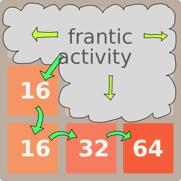
Further rightward merges create a 128 in the bottom right corner.
[Simon Tatham, 2026-09-09]
A few years ago, the puzzle game 2048 was popular. I found it fun, but a bit too long. I wanted a shorter version of the same game, so that I could more easily squeeze in a quick play while waiting for something else to finish, like a long compilation.
The obvious answer is to play it on a smaller grid than the usual 4×4 one. The standard implementation didn’t have an option for that, but the game rules are simple, so I wrote my own version. Here, you can have a go yourself:
But changing the grid size surely means changing the target number. What’s a reasonable size of tile to expect players to be able to make, on a 3×3 board?
I could have come up with an answer to that question by extensive play-testing, alone or with friends. But I had a different idea. The 3×3 version of 2048 is small enough that you can reasonably iterate over all possible states of the board. So I could analyse the game to find out how well a perfect player would do, and base the choice of target on that.
So I did that. In fact I did it in 2018, and I’m only just now getting round to writing it up. Sorry!
Normally I avoid using any Javascript in blog posts like this, because I’m sympathetic to people who want to keep it turned off, to avoid both security hazards and intrusive behaviour of web pages. In this article, I’ve made a rare exception, because I wanted to present inline applets for playing the game, and also I couldn’t think of any sensible non-JS way to show a full replay of a perfectly played game. (My usual technique for image flipping in pure CSS is all right for half a dozen images, but not 500.)
So I’m afraid that if you were to read this article without Javascript, you’d miss out on some of the most fun parts. Sorry about that!
I had two reasons to think that 3×3 2048 would be an easy game to analyse exhaustively.
First, as I mentioned above, the state space is manageably small.
Suppose you want to know the probability of a perfect player successfully making some particular tile value 2k. In that case, on your 3×3 board, you expect that each cell is either empty, or contains a tile with one of the k values 2, 4, 8, …, 2k. So there are k + 1 possible states that a cell can be in, and 9 cells overall, giving a total state space of size (k + 1)9.
Even if you’re ambitious enough to want to make the original target number of 2048 = 211, that still only gives you 129 possible game states, which is not much more than 232. There’s no difficulty for a modern computer doing a calculation for each of that many states. It doesn’t even take very long – seconds or minutes, not even hours.
Secondly, 2048 is monotonic: in every move, the sum of all the tiles on the board strictly increases. That means no game can ever return to a previous position. Therefore, there’s no possibility of the game continuing forever, or having to determine the values of positions by solving a complicated system of simultaneous equations. Either of those would complicate an analysis, and neither one can happen.
Before describing how a program solves this problem, we should state precisely what the problem actually is.
The basic idea in this kind of work is to associate to each board position a value. Values can represent various detailed things depending on the game (probabilities, scores, simple yes/no questions about which player is in a winning position), but whatever the details, the value of the current game position should be the thing the player is aiming to maximise. In this case, because I’m interested in the question “What’s the probability of the player successfully making a particular target tile?”, it makes sense to have the value be that probability.
In fact, in 2048, we have two probabilities associated with each position:
In my analysis code, I called these the pvalue and cvalue respectively, named after whose turn it is in each case.
The rules for calculating these values are:
This isn’t quite the same as the way two-player games are normally analysed. More usually, one player aims to maximise the value of the game and the other player aims to minimise it. But in 2048, the computer isn’t playing against you on purpose, choosing the tile drops in order to try to make you lose. It’s just picking one randomly. So here, the player maximises the value while the computer just takes the (appropriately weighted) mean value over all its possible moves.
Finally, our real question is not about the value of one particular game position. It’s about the value of the whole game: what’s the chance of a perfect player making the specified target tile overall? To answer this, we must calculate the average pvalue over all the possible starting positions (pairs of initial tile drops).
That’s a mathematical statement of the problem. Now what’s a good algorithm to solve it?
Each board position has a pvalue and a cvalue associated with it, and we’re trying to calculate them. For most positions, in order to calculate these values, you need to know the values of other positions later in the game – in particular, with their tiles summing to a larger number.
There are essentially two approaches, both with the property that you never calculate the value of a position more than once:
The tradeoff between these two approaches is that recursion comes with a risk of overflowing the stack, but dynamic programming must evaluate every position, not just the positions that can be reached in legal play. So DP is likely slower, but recursion might not work at all.
In this case, recursion is fine. 2048 games only go on for a few hundred moves, and that’s not enough to overflow the stack of an ordinary Linux application. So I went with that approach.
I also didn’t bother caching both the pvalue and cvalue for each position. Caching just one is enough – I chose to cache the pvalues. That means the cvalue function still needs to repeat some work if it’s called more than once on a position, but not much, because the second time, all its calls to the pvalue function will return immediately. So you lose a little bit of speed, but the risk of running out of RAM (in which case the program won’t give any answers at all) seemed more important.
One possible optimisation I could have done, but didn’t bother with, is to reduce by symmetry. 2048 is essentially symmetric: if a position is rotated or reflected, then it shouldn’t make any difference to the probability of winning, because all the same moves and drops are legal in the rotated position – or rather, their corresponding rotations/reflections are legal. So I could have normalised every board position into a canonical orientation (say, by calculating all 8 rotations and reflections of it, and picking the one earliest in some sorting order).
The advantage of this is that the evaluation functions would have run on about 1/8 as many positions – a typical position is completely asymmetric, so 8 transformed versions of it all have the same value, and we could have reused the result of the first of those calculations for the other 7.
On the other hand, the normalisation itself would be extra work. I don’t know whether this would have been a net win overall.
And it would have made the code more complicated, which is also a cost. The simple version of the code was already fast enough, so I didn’t even bother trying this.
Finally, how are these pvalues and cvalues represented, inside the analysis program? They’re probabilities – real numbers between 0 and 1 – so the natural data type to use is floating point. In fact there’s not really any other practical choice. But floating point isn’t completely accurate, so is there a possibility that rounding errors confuse the calculations?
Indeed there is, and I’ll come to it in the next section.
I wrote this program in 2018 and ran it. The headline results, with perfect play, are:
So I decided that 256 is a reasonable tile to take as the standard game target, because if you fail to make it, it’s almost certainly a skill issue – a perfect player would succeed very nearly every time. Then, if you have motivation and time (e.g. that compilation still hasn’t finished), carrying on to make a 512 is a good stretch goal: you might manage it, and you can feel good if you do, but if you fail then you don’t have to feel too bad, because there’s a decent chance it was just bad luck.
The probability of zero for making a 2048 tile suggests that it’s literally impossible. On the other hand, maybe it’s a floating-point rounding error, and the true probability is not quite zero?
But no, making a 2048 tile on a 3×3 board really is completely impossible, and the proof is reasonably simple:
There’s no probability in this proof at all. It doesn’t depend on the random drops actually being random. It would still be impossible to make a 2048 tile even if the random drops weren’t random – even if you were allowed to choose them, to suit yourself perfectly.
Of course, this means that calling this game variant “3×3 2048” is a misnomer, since making a 2048 is one thing you definitely can’t do in it! But it can’t be helped. If you call it anything else, nobody will know what you’re talking about.
What about that tiny probability of making 1024? Why’s that so amazingly hard?
Well, suppose we follow the same proof again, divided by 2. That is, we start from the premise that someone has managed to make a 1024 tile, instead of a 2048. Going through the proof in the same way shows that at some point in the game there must be a position in which all nine tiles are at least 4. And, again, one of those tiles has to be the most recent random drop.
This time it’s not impossible – sometimes random drops are 4s! But it’s unlikely, because only 1/10 of them are 4s. So to make a 1024, you have to go to all the effort of setting up the right conditions so that if that crucial drop is a 4 then you can win … and then, nine times out of ten, the drop is a 2 instead, and you lose, and there was nothing you could do about it. Arrrgh.
The probability of getting everything in place before the crucial drop is about 11.3%. That’s harder than making a 512, but not absurdly hard. But then that drop itself reduces the probability of winning by another factor of ten.
I think, if I wanted to make 1024 a reasonable goal for a dedicated player, I might make the game cheat very occasionally in the player’s favour: somehow identify that specific situation in which you’ve done everything right but now you need the drop to be a 4, and in that one case, make sure you always do get the 4 you need.
(How would you characterise that situation? Well, a small extension to the above proof demonstrates that to make 1024 you need to pass through a state in which not only do you have nine tiles all ≥ 4, but also the sum of the nine tiles is at least 1024 – for example, eight of the tiles run from 4 to 512 inclusive, and the ninth is a second 4, so that you can merge all nine down to a single 1024. So I’d force the drop to be a 4 when it would otherwise just miss creating that more specific situation.)
What about tiles smaller than 256?
When I ran this calculation in 2018, it reported that the probability of making a 128 tile was 1. (Or 100%, if you prefer.)
That means it ought to be unconditionally possible, no matter how unlucky you get with the random drops. Another way of putting that is that if the random drops were instead controlled by a perfectly-playing adversary – let’s call it “Satan” – which was doing its best to prevent you from making a 128 tile, then with perfect play of your own, you’d be able to make a 128 in spite of everything Satan could do to stop you.
But this isn’t true! Unlike the case of the 2048 tile, where the probability of 0 was literally exactly zero, this probability of 1 is not literally 1. It’s a floating-point rounding error.
In 2018, I did this calculation storing all the probabilities
in single-precision floating point: the float type
in C, 32 bits wide. The float type can represent
numbers to about 7 decimal places of precision. In particular,
the largest number it can represent that’s less than
exactly 1.0 is about 0.99999994. If a number is closer to 1 than
that, it might well be rounded up to 1.
This year, repeating the calculation for this writeup, I had
more RAM available, and so I used the 64-bit double
type instead of float, just to see if it would make
a difference. And it did. The double version of the
analysis reported that you can make a 128 tile with probability
only about 0.9999998 (or 99.99998%). Definitely not
exactly 1.
(You might notice that that value isn’t closer to 1
than 0.99999994 is. There’s one fewer 9 after the point. It’s
actually several notches away from 1, in the minimum increments
that float can distinguish. But it was the result
of a long calculation involving many operations, so there was
more than one rounding error involved, and I have to assume that
it rounded up more than once.)
A good way to get round this problem turned out to be to flip the sense of the value. Instead of calculating the probability of the player succeeding at making a 128 tile, we instead calculate the probabliity of them failing (and then of course the player chooses a move to minimise rather than maximise that value). Floating-point numbers are bad at representing numbers very close to 1, but excellent at representing numbers very close to zero, so we can get much more precise figures for the easy end of the scale:
This time, that last zero is literally zero. You really can make a 32 tile even if Satan has taken over the random drop generator and is going all-out to prevent you.
But Satan can stop you making a 128, and even stop you making a 64. You’d have to get astronomically unlucky to be unable to make a 64 with the standard random drops – but if Satan is choosing the drops on purpose, you’ll fail every time.
It’s all very well to list the winning probabilities for perfect play. But that’s not all we’d like to know. We’re naturally curious to know what perfect play is!
Our algorithm for calculating the winning probability works by calculating the pvalue for each board position, and the problem definition specifies that the pvalue is obtained by considering every possible move, and choosing the one that leads to the position with the best cvalue. So our existing algorithm is already working out what the best move is in every position. All we need to do is to make it save that list of ideal moves, as an extra output in addition to the win probability.
This gives us a complete description of perfect play (for a particular target tile). But it’s in the form of a gigantic lookup table. How do we start getting any understanding from it?
My answer was: modify my implementation of the actual game so that, instead of getting input from the user to decide what move to make, it can use the lookup table output from the analyser. Then you can watch example perfectly-played games, and learn from them in the same way you might learn from watching a more skilled human player than yourself: notice when it did something that wasn’t what you’d have done, and think about why, and try it yourself to see if your play improves.
Here’s an example game, derived from the strategy table for making a 1024 tile. As we saw in the previous section, even a perfect player only expects to manage this about one game in 100. But it takes almost no time to try 100 games until one succeeds. So here it is:
What insights you get from watching that replay will depend on what your play was already like. In my case, the main thing I learned was to use a strategy based on one corner of the board, instead of one edge.
When I first started playing 3×3 2048, I used the same basic strategy as I used for 4×4, which is the same strategy as everyone else I’ve ever discussed the game with. That strategy is to keep the high-value tiles along one edge of the board (I habitually use the bottom row), in increasing order from one end to the other (I do it left to right). Then use left, right and down moves to construct tiles you can merge down into the bottom row.
The new strategic concept I learned from the perfect player is to instead keep your high-value tiles in a 2×2 block in one corner of the board – I habitually choose the bottom right corner. Usually the very highest one goes in the very corner, with the next two highest on the edges, and the lowest of the four in the middle. Then, as long as the squares to the left are blocked, you can slide left and right to manipulate the top row, without moving the high-value corner tiles out of place. And then you can switch to sliding up and down to manipulate the left column, and between those two operations, make something you can merge into the centre tile, and then merge that into an edge, or out of one edge into the other.
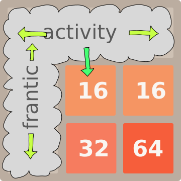
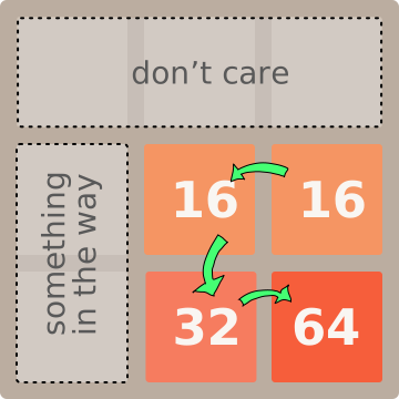
The automated player doesn’t rigidly stick to this style. (Surely part of its edge is that it doesn’t insist on rigidly sticking to any style, and can be flexible as the need arises.) But you can see reasonably clear examples of the corner-based playing style in the replay above, most obviously when it’s just leading up to make a new highest-value tile. For example, moves 105–126 when it’s about to make a 256; moves 214–246 when it’s about to make a 512; and moves 425–472 when it’s getting everything ready for the final push to a 1024. In the first two of those segments its high-value corner is in the top left; by the third segment it’s found some need to change its point of view, and now it’s using the bottom left.
After I saw the auto-player using this strategy, I started trying it myself. It took a while to get the hang of it – the basic idea is simple enough, but there was a new set of details to learn, about all the tricks you can use in the free row and column. But it was definitely an improvement, once I’d learned those tricks. Before changing strategies, I’d been able to make a 512 tile about twice ever. Afterwards, I got them on a fairly regular basis, and occasionally in two successive games. I’m sure my play still wasn’t perfect, but that one lesson was worthwhile!
Why is this strategy better than the one I was using before? That’s not generally an easy question to answer; in fact there’s no real guarantee that there even is a nice short easy-to-understand answer. But I do have one thought.
The big weakness of the bottom-row strategy, in general, is that you can only use left, right and down moves. You never want to move up. If you find yourself forced to, it makes a really horrible mess, and you might not be able to collect all the high-value tiles together again.
But the corner strategy can use all four directions! You can slide the left column both up and down (as long as the spaces above the high-value corner are full), and you can slide the top row both left and right (as long as the lower left spaces are full). So you make better use of the available moves, and give yourself more options.
A couple of other things to note in the 1024 replay above:
We proved in a previous section that any successful creation of a 1024 tile must pass through a previous board state in which all nine tiles are at least 4 (and I also added that the tiles must already sum to 1024 at that point). Here, that happens at move 467. The previous move had two 2s in the top left corner; it slid right, merging them into a 4, and a new 4 appeared in the top left corner as a random drop (with 1/10 probability, of course). Now the board contains every power of 2 from 4 up to 512, and the ninth tile is another 4. So you can merge the 4s into another 8, merge the 8s into another 16, and so on until you have a second 512 to merge into the existing one, and you’re done!
But in fact that’s not what the auto-player does. It merges as far as having two 256 and a 512, on move 473 … but then for some reason it stops and faffs around doing other stuff, until move 479, when it seems to suddenly remember what it was supposed to be doing, and finishes up the sequence of merges that make the 1024 and win the game.
Why did it stop and faff about? Simply because nobody told it not to.
The optimiser was given just one criterion: pick the move with the best probability of making a 1024. But it doesn’t have any kind of tie-breaking criterion. So if two moves both have 100% probability of making a 1024, it has no reason to pick one over the other. It won’t do the common-sense thing a human would do, of picking the move that makes a 1024 soonest. It’ll just pick whichever of the moves it found first while iterating through them all!
The analysis technique I used in this project is fundamentally based on having a fixed goal. When we calculated the probabilities of making 256, 512 and 1024 tiles, each one of those was a totally separate calculation, delivering a completely different lookup table of strategy.
But when a human plays this game, they can change their goal. As I suggested above, your primary goal in the game might be to make a 256, and then, after you’ve succeeded, you might decide to play on and make a 512.
What happens if you tier the optimal strategies in the same way? If you use the 256 strategy to maximise your probability of making 256, and then see what the 512 strategy can do from the end position, how well does that do?
It’s easy to imagine that that might not do as well as if you’d used the 512 strategy consistently from the start of the game. For a start, you certainly wouldn’t expect it to do better, because the dedicated 512 strategy is supposed to be the best possible! But also, while you’re following the 256 strategy, your only goal is to end up with a 256 tile, and not to leave the board in a suitable state for followup play. So you could imagine the 256 strategy having left a disadvantageous position for the 512 strategy to take over from.
On the other hand, it surely can’t be too disastrous. When you make a 256, you’ve just merged together most of the tiles on the board, so what’s left will be recent random drops, probably easy to merge together in turn. So perhaps you don’t expect too much of a reduction in winning probability.
It turns out that you lose about 1%. The best possible strategy for making a 512 tile succeeds 73.7% of the time; if that strategy takes over after the 256 strategy finishes, then that goes down to 72.6%. Not too bad.
What about the other way round? If we just run the strategy for making the biggest possible tile (a 1024), how much does it hurt our chances of making the smaller tiles?
The answer is: much, much less. The probability of making a 512 using the 1024 strategy is lower than the dedicated 512 strategy by about 10−7, and the chances of the lower tiles in turn go down by similarly small amounts.
However, the 1024 strategy can fail to even make a 32 tile! It fails with probability less than 10−14, but that’s not zero, and we know it is possible to make a 32 with 100% reliability.
So, in principle, there’s no one strategy that combines the maximum probability of making every value of tile. You’ve always got to trade off something. But in practice, the top-tier strategy that can make a 1024 is so close to also being the best at everything else that you might as well not worry about it!
I said earlier that, because 2048 chooses the tile drops at random, the cvalues are calculated as a mean over all the possible drops, instead of a minimum.
Suppose we calculated the minimum instead? Then we’d switch to treating this game as a proper two-player game, between one player choosing the moves and an opponent choosing the drops.
In this version of the analysis, you don’t need to store floating-point probabilities, because there’s no randomness being modelled. As a two-player game, 2048 is deterministic. So pvalues and cvalues become single bits: either 1 for ‘the move player wins from this position’ and 0 for ‘the drop player wins’.
(This is how I double-checked the claim in a previous section that the probability of failing to make a 32 was literally zero. To rule out the possibility of further floating-point rounding errors, I did the analysis in a way that doesn’t involve any floating point. Now I’m confident that even if I upgraded to an even larger floating-point type like 128-bit quad precision, there still wouldn’t be any nasty surprises.)
But also, running the analysis in this mode means that we’re choosing the best move for the drop player in each situation. So, just as we did for the move player, we can extract the drop player’s best strategy as a by-product of the analysis.
I said earlier that if Satan was choosing the tile drops, you couldn’t make a 64 tile. This technique allows us to figure out the exact strategy Satan would use to prevent you from doing so.
In fact, I can demonstrate it right here! Here’s an instance of the game in which you are playing against Satan.In this game, the drops are still randomised, so that it won’t play exactly the same every time. It’s just that the drops are chosen at random from a subset of all possible drops: the ones from which Satan still has a winning strategy and you don’t.
You should find that it’s impossible to make a 64 tile in this version of the game, no matter how hard you try. But that’s the only constraint Satan is enforcing. It is possible to make a pair of 32s, but you’ll find you can never quite get them next to each other. The best set of tiles I’ve managed to create at all included two 32s, two 16s, and an 8.
I started this entire project just because I wanted to know what was a fair target number to require of the player on the 3×3 board. But I got more than that out of it!
I learned a whole better way to play the game, and had a lot of fun re-training myself to play in that style. I learned some new and exciting gotchas about exhaustive analysis of games – the next time I’m forced to use floating-point probabilities, I’ll try both win and loss probabilities much earlier in the exercise. And even the version of the game playing against Satan is kind of fun, in a perverse, masochistic sort of way.
And I still have some unanswered questions, which is also a sign that a problem domain is interesting.
First, are these ‘optimal’ strategies really optimal? Since we’ve already seen that the use of floating point introduces error, is it possible that these strategies are actually choosing a non-optimal move in some situation, because enough errors have built up in calculating two successor positions’ values to make the wrong one look larger? It’s clear that the strategies output from my existing code are pretty good: in particular, the strategy I calculated for making a 1024 tile can successfully do that job, because I didn’t have to wait long for the auto-player to spit out a game history in which it succeeded. But maybe it’s still not quite the best?
Second, is there any analogue on the original 4×4 board of the ‘high-value corner’ strategy that this exercise taught me for the 3×3? I’m not sure it would work as well there. If you made the high-value corner a 2×2 block of the whole 4×4 board, then it’s harder to get it properly blocked into one corner so as to be able to move everything else around. But if you make it a 3×3 block, then it’s harder to move things within the block. This might be a strategy that only works on the smaller board, and doesn’t scale.
One last thought:
I said at the start of the article that I didn’t like 4×4 2048 because it takes too long to play, and wanted a shorter version that wouldn’t use up so much of my time. But I’d overlooked something. If you know that ‘just one quick game’ won’t take very long, you have a lower barrier to choosing to play it at all – I’m willing to have a quick 3×3 game in situations where I wouldn’t have even started a 4×4. So, even if you don’t count the part where I got nerd-sniped by the analysis project, I’m not sure I actually did end up reducing the amount of time I spent playing 2048!
With any luck, you should be able to read the footnotes of this article in place, by clicking on the superscript footnote number or the corresponding numbered tab on the right side of the page.
But just in case the CSS didn’t do the right thing, here’s the text of all the footnotes again:
1. You could call this a “meanimax” analysis instead of a minimax one. But I won’t. It sounds enough like the usual word to be confusing!
2. I once saw a clone website that did let you scale the game down to 3×3, and it kept 2048 as the target tile. Perhaps they hadn’t realised it’s impossible. But the site was also extremely covered in adverts, so another theory is that they were deliberately setting you an impossible task to keep your eyeballs there as long as possible!
3. If I had done the ‘reduce by symmetry’ optimisation from the analyser as I suggested above, then this part of the job would also have become more complicated, because I’d have to keep track of which orientation of the canonical version of a position matched the one in the current gameplay, and translate all the moves accordingly. And that orientation might change between moves!
4. You could also imagine redoing this analysis with a more quantitative optimisation goal than ‘try to make a 512’. You could aim to maximise the expected sum of all the tiles. Or to maximise the expected score as calculated by the original game, which I think is the sum of all the tiles created in merges, regardless of whether the tile was later consumed by another merge. These kinds of goal will also work out to be maximising for some kind of weighted combination of the more primitive goals like making a particular high-value tile.
5. In fact, in this case, it’s cheaper to extract the table of pvalues than the table of best moves, because that way the data file is smaller. This wasn’t true when pvalues were floats, because a float is larger than a description of a move. But here, a single-bit pvalue is smaller than a description of a drop. With this approach, and knowing that only tiles up to 32 can appear at all, the strategy data file for the game in this section only needs to be 69 bits long, i.e. about 1.2 MB. Then the software must choose a drop by looking up the pvalue for every possibility, and choosing from the ones that don’t give the player a winning strategy. But that’s still more than fast enough.