[go back to the main polyhedral pictures page]
To create my polyhedral globes, I started off with the GTOPO30 data set from the US Geological Survey.
GTOPO30 is conceptually an enormous rectangle of raw bitmap data. Its x-coordinate runs from longitude 180°W to 180°E in steps of 1/120 degree, and its y-coordinate runs from latitude 90°N to 90°S in the same increments. So the entire bitmap is 43200×21600. It has 16 bits per pixel, which are a single 16-bit integer giving the ground elevation in metres above sea level for that position on the globe. The special value -9999 indicates sea. (So the data set distinguishes between sea and ground that's below sea level: negative values other than -9999 exist, for example in the Caspian Sea.) Instead of a single 1.7Gb data file, the data is divided into 33 smaller rectangular tiles.
Converting that source data into a spherical image was basically a long job of step-by-step transformation.
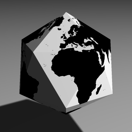
I began with a black-and-white globe, which simply distinguished sea from land. So my first job here was to convert the 16bpp bitmap described above into a 1bpp bitmap, in which each pixel either denoted "land" or "sea". This is a simple matter of streaming data processing.
My method of defining spherical images is basically vector-based, so
the next step was to convert that bitmap into a set of vector data
which drew round each coastline. For this, I used an existing
tracing program,
potrace.
Since I wanted to end up with relatively small chunks, this was also a good moment to divide the large bitmap into sufficiently small pieces and trace them all separately – not forgetting to ensure a small amount of overlap between the pieces, to avoid potential rounding error if two regions of blackness exactly shared a boundary. (There's always the risk that PostScript's floating point processing might happen to round the boundaries in opposite directions, so you might end up with white pixels at the joining line. Ensuring a small overlap solves this.)
Also during the tracing phase, I had to select my resolution. My globes were not actually generated from the full-resolution GTOPO30 bitmap; that would have made all the coastlines much more complex, and hence bloated the size of the output PDFs, for little or no visible benefit. So I had to choose a factor by which to shrink the bitmaps before tracing, so as to best trade off file size against detail. I ended up shrinking them by a factor of 10.
After that, I had to take all my pieces of plane vector data, convert them back into spherical coordinates, and restore them to their correct places on the globe. Having done that, I had a spherical image describing my black and white globe!
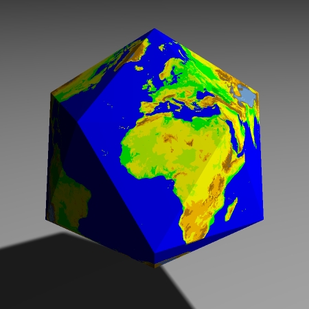
For the colour version, I simply repeated the entire procedure several times, with the only difference being that the initial reduction from 16bpp to 1bpp was done by setting a different elevation threshold for each layer. Thus, I ended up with a set of dark green polygons describing land, then a set of lighter green polygons describing all land higher than 200m, lighter still for land higher than 400m, and so on. Then I overlaid all those polygons (in the right order, of course), and there was my coloured globe. No additional conceptual difficulty, just a matter of running the same program several times with a different argument.
[go back to the main polyhedral pictures page]
(comments to anakin@pobox.com)
(thanks to
chiark
for hosting this page)
(last modified on Sun May 7 14:33:22 2017)